Introduction
Black Holes
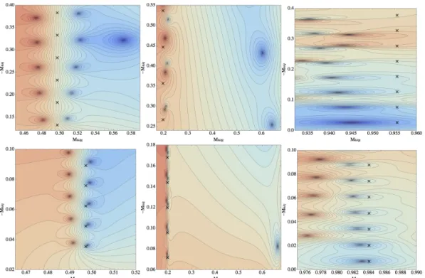
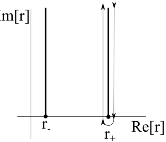
The zeros of the continued fraction (seen above as a cluster of contours in a dark region) are QNM frequencies, and are usually accompanied by a pole nearby (a cluster of contours in a lighter region). A muted mode is also visible to the right of the ZDMs in the top panel.
The Quasinormal Modes of Weakly Charged Kerr-Newman
Abstract
These modes, called quasinormal modes, play a central role in determining the stability of Kerr–Newman black holes and their response to perturbations. The new formalism reveals no unstable modes, which together with previous results in the slow-rotation limit strongly indicate the modal stability of the Kerr–Newman spacetime.
Introduction
Our first-order calculations show no unstable modes, which, when complemented by the slow rotation study [Pani2013PRl,11], provide strong evidence for the linear stability of the KN spacetime. In addition, we provide the first analysis of the near-extremal Kerr-Newman (NEKN) QNM frequencies in the rapidly rotating regime.
QNM frequencies of weakly charged black holes
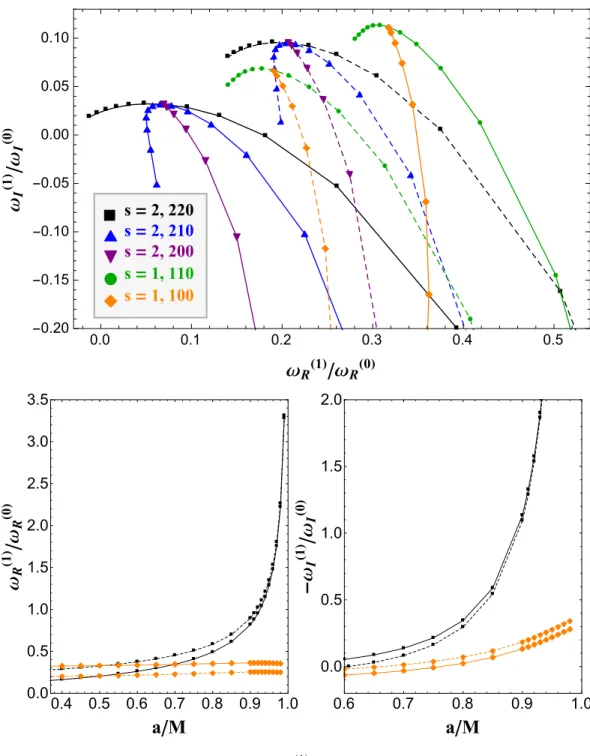
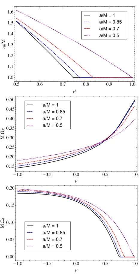
Note that asa→ M, the DF equation predicts an increasingly accurate correction of the frequency ω(1) for the mode thes = 2, 220, but not for the mode thes= 1, 100. 2.5), we can understand this phenomenon in analytical way. Almost Extremal Kerr-Newman.—We now consider the modal stability of the weakly charged NEKN spacetime (q < qmax=2 −2 1), where we have 2.9) Numerical investigations and near-extremal expansions [31] reveal that the extremal DF equation predicts stable marginal modes (ZDM) for any value of Q , whereas previous work has not found ZDM in RN space [32,33] .
Future Work
To estimate how large Q can become before higher-order contributions (in q) become significant, we use the EVP method to calculate the leading-order correction ω(1) to the QNM frequencies of the DF equation. According to our intuition from Figure 2.3, confirming the existence of such a mode would require knowledge of the higher-order charge correctionsqjω(j), which can also be measured as O(√.
Acknowledgments
Finally, our analysis of NEKN black holes raises the question of whether ZDMs exist for near-extreme black holes of arbitrary charge, which can be addressed by a more complete NEKN analysis. This would be complemented by the WKB analysis of the coupled equations (2.1), which would give further insight into the KN QNM, the existence of ZDM and DM, and the possible geometric correspondence of the QNM with the geodesic [30,34] and tem = 0 wave equation in the KN.
Appendix: The Perturbed Kerr-Newman Spacetime in the Newman-
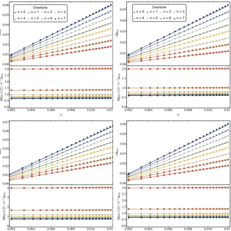
This analysis is a straightforward generalization of the results discussed in [36], and was also recently presented in [43], which focused on the connection between the WKB frequency formulas and the behavior of unstable null geodes at the light sphere (see also [21]). The O(σ)2 scaling of the residuals stops short enough σ, as discussed in the text.
Damped and zero-damped quasinormal modes of charged, nearly-
In this study, we investigate the existence of families of quasinormal states of Kerr–Newman black holes whose decay rates limit to zero at the extremity, called zero-damped states in previous studies. These results, together with recent numerical studies, point to the existence of a simple universal equation for the frequencies of zero-damped gravito-electromagnetic modes of Kerr–Newman black holes, whose precise form remains an open question.
Introduction
In particular, Kokkotas and Berti studied QNMs of the Dudley-Finley (DF) equation on KN backgrounds [20, 21]. Thus, analysis of the bag equation =0 DF gives the true scalar QNMs of the black hole KN.
The Dudley-Finely equation for nearly-extremal Kerr-Newman black
Both the matched asymptotic expansion and Kerr's WKB analysis apply directly to the case of the DF equation in KN. To confirm the WKB predictions for the QNMs of the DF equations, we calculate the analytical ωA by solving Eqs.
Gravito-electromagnetic modes of Reissner-Nordström
To analytically search for ZDMs in the NERN spacetime, we repeat the steps of the corresponding asymptotic expansion used for the DF equation in Sect.3.3. In the case of the DF equation in NEKN, the ZDM solutions correspond to the near disappearance of one of the two coefficients of (σ/x)1/2±iδ in the above expansion.
Conclusions
Importantly, our analysis establishes the existence of ZDMs of the GEM perturbations of RN black holes for the first time to our knowledge11. The dependence of the ZDM frequency (3.37) on spin and charge also explains the frequency behavior seen in the numerical simulations presented in [30], as pointed out in a remark by Hod [44].
Appendix:Details of the matching calculation
Here we have normalized each amplitude to the amplitude of the horizon wave function, Zhole. For this we transform the domain of the hypergeometric function 2F1 taking z=1− yand using the identity [51].
Appendix: The WKB analysis of the Dudley-Finley equations
The modes of the ECO spacetime come from the poles of the response function K(˜ ω) appearing in the Green function. The fundamental limit of the detector sensitivity is determined by the quantum noise (gray trace) and the thermal (blue trace) noise [1].
A recipe for echoes from exotic compact objects
Abstract
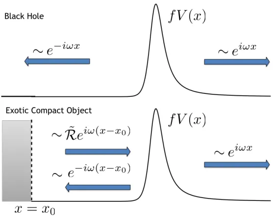
We show how to reprocess radiation in the near-horizon of a Schwarzschild black hole to the asymptotic radiation from the corresponding source in an ECO spacetime. We find that the quasinormal mode ringing in the black hole spacetime plays a central role in determining the shape of the first few echoes.
Introduction
In Section 4.4, we show how the additional part of the ECO waveform can be expressed as a sum of echoes. In Section 4.6, we determine the general properties of individual echoes and develop a simple template for the ECO waveform.
Waves near a compact object
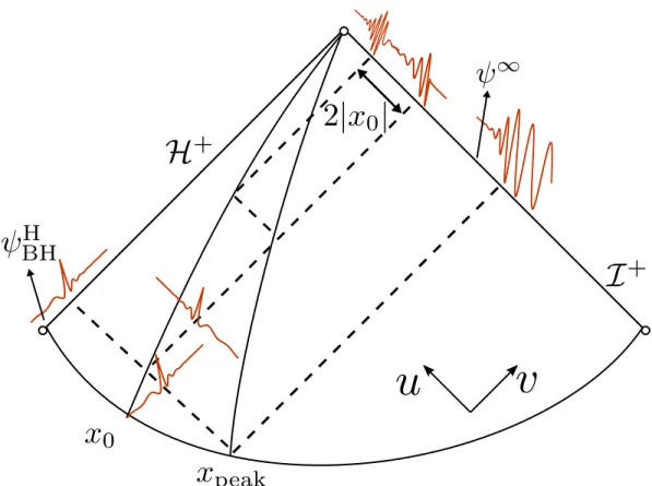
Having defined these amplitudes, we can, in the presence of the reflecting boundary ˜greff from Eq. 4.11) to calculate the asymptotic amplitude associated with scalar waves ˜ψ,. This shows that the waveform seen by distant observers can be understood as the sum of the ordinary emission in a BH spacetime, together with an additional signal ˜KZBHH.
Examples of Echoes
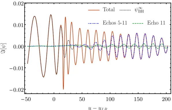
As expected at low frequencies compared to the magnitude of the potential peak(Mω)2Vp, waves are completely reflected. A comparison of the first echoes and the fifth echoes produced by a test charge following the ISCO dive trajectory is shown in Fig. 4.8.
Excitation of ECO Modes
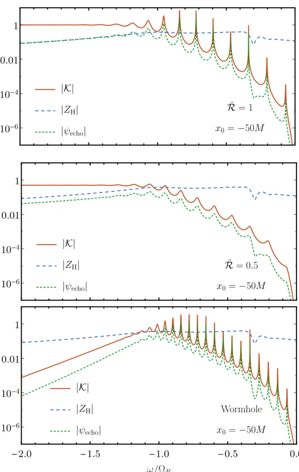
This scenario can also be understood from the additional resonances of ECO spacetime. The horizon amplitude is significant at all the resonances of ˜K, which have spacing ωFSR.
General Features of echoes
4.20 shows that the template has important features of the horizon waveform at low frequencies|ω| misses <ΩR. For perfectly reflective, extremely compact ECOs with x0 > 20M, more than 97% of the energy in the horizon waveform is radiated in the echoes.
Conclusions
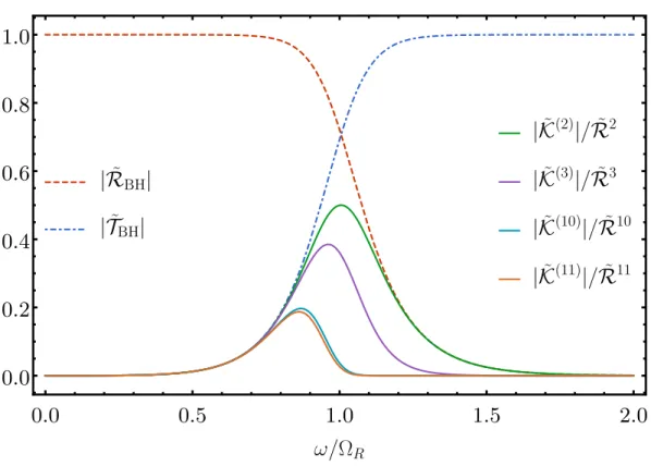
Despite the imprint of these frequencies on the ECO waveform, our formalism also shows that the BH QNM frequencies are not poles in the ECO Green's function. On the contrary, the part of the Green's function responsible for producing the main burst and the part responsible for the echoes both have poles at the BH QNM frequencies, which cancel in the full expression.
Our formalism also explains how BH QNMs are imprinted in the ECO waveforms: the ECO waveform has a main burst ringing down at QNM black hole frequencies. Furthermore, the frequency content of individual echo pulses is largely determined by the frequency content in the ψBHH horizon waveform near the BH QNM frequencies.
Appendix: Calculation of the reflection and transmission coefficients 105
Similarly, we extract TBH from rayv =vE in our computational domain closest to I+. We verified that the same numerical approximation of δ(u) that we used in our initial data appears in TBH.
Appendix: Point Particle Waveforms
Equation (4.80) together with initial data ˆg=−1/2 on the future part of the zero cone formed by raysu= u0 and v = v0 is a characteristic initial value problem forgBH. We generate values for ψ at the remaining nodes of the lattice using the stepping algorithm (4.81).
Appendix: Wormhole Reflectivity
We obtain the horizon waveform ZBHH in the frequency domain by numerically performing the inverse Fourier transform of the time domain waveform ψBHH. In the left half of the universe, ˜ψup(−y) is the solution that describes waves that are completely outgoing at zero infinity.
Appendix: Fourier Transform of Decaying Sequence of Pulses
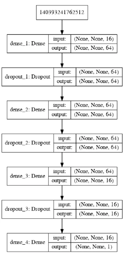
For example, in the bilinear noise mechanism, the spot displacement ∆y and the mirror angular motion ∆θ are witness channels and the length change ∆Li is the target channel. Let's say the output of the previous layer has shape (number of time steps, number of channels), then the output of the convolutional layer will have shape (number of time steps, filter number).
Noise Subtraction with Neural Networks
Subtractable Noise
The inspiratory fraction of binary neutron star mergers, which is necessary for early warning detection of the mergers, also falls in the sub-100 Hz regime. In the 10-20 Hz band, the measured noise (red trace) is almost two orders of magnitude larger than the sum of the quantum and thermal noise.
![Figure 5.1: Noise budget of aLIGO [1]. In the sub-100 Hz band, the sensitivity is limited by subtractable noise sources since the measured noise (red trace) is up to two orders of magnitude larger than the unsubtractable noise sources, the quantum (gray tr](https://thumb-ap.123doks.com/thumbv2/123dok/11054124.0/147.918.179.747.138.541/figure-sensitivity-limited-subtractable-sources-measured-magnitude-unsubtractable.webp)
Mock Data
The angular witnesses are essentially ASC error signals that measure the hard and soft states of the mirror rotation, which differ from the true angular motion by a 1/f4 transfer function of the suspension. We model the true spot position as a linear combination of the eight ASC error signals (again multiplied by another mixing matrix to model cross-couplings and supplemented with white measurement noise) and eight ISI channels (supplemented with measurement noise) plus and unknown DC offset.
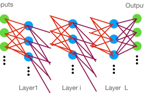
Neural Networks
In regular gradient descent, the gradient of the cost function with respect to the weights∇vC is calculated and the weight is updated as . To achieve this, we always use a smoothed rate of `0.5 to adjust the weights in the EQL layer.
Mock Data Results
Each node in the comparison layer has a (potentially different) activation that is common in physical models. Even if we had the optimal neural network, we would not obtain a perfect subtraction due to measurement noise included in the colored bilinear mock data.
Conclusion
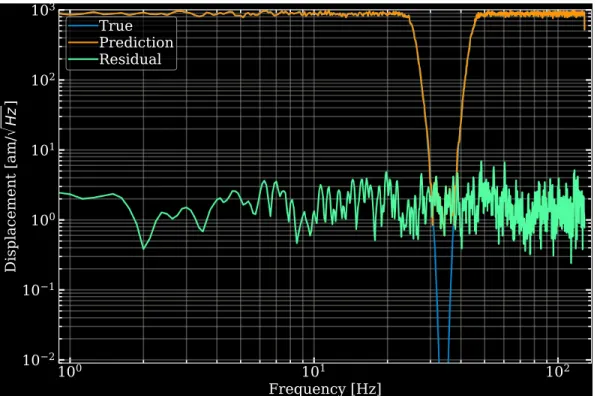
We managed to solve the most realistic bilinear mocks with a network that relies on 1D convolutional layers to learn frequency-dependent filtering and EQL layers to learn nonlinear couplings. Figure 5.12 illustrates the successful subtraction by showing the spectral amplitude densities of the target, prediction, and residual.