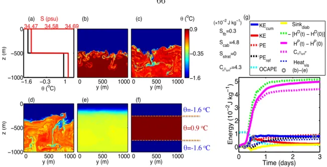
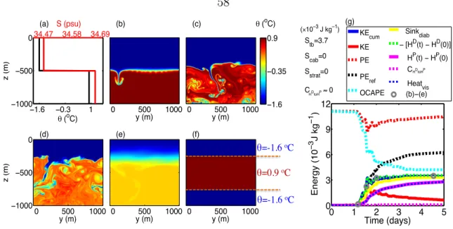
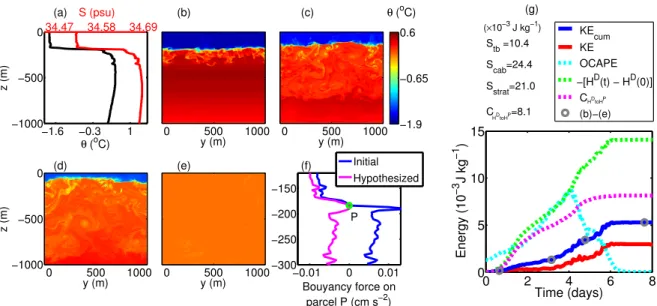
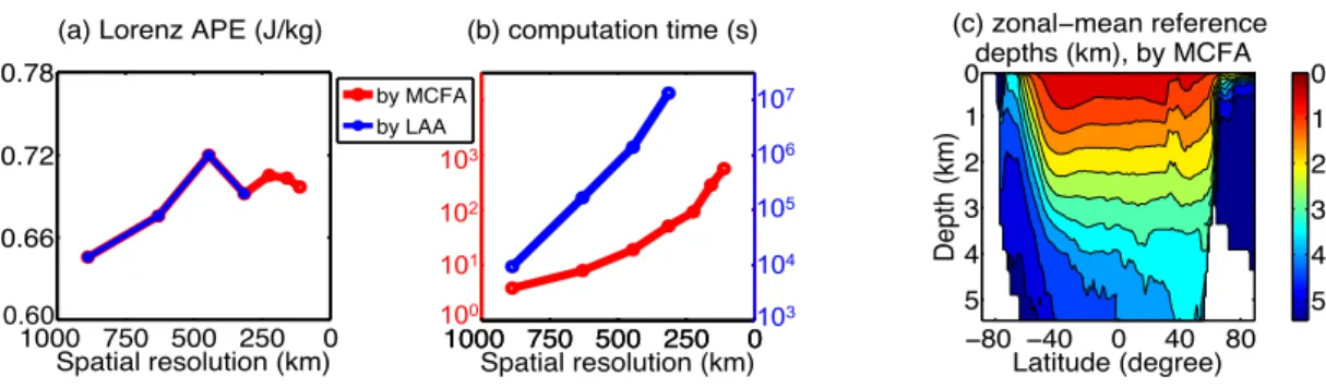
Here z and y are the vertical and horizontal coordinates, respectively. f) Reference state (minimum PE) for the initial profile. g) Energy budget time series (curve). From (a), the solution converges with increasing resolution. c) Average zonal depth (km) where the current state plots lie in the Lorenz reference state.
Case 1
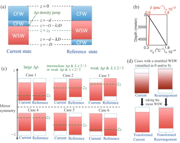
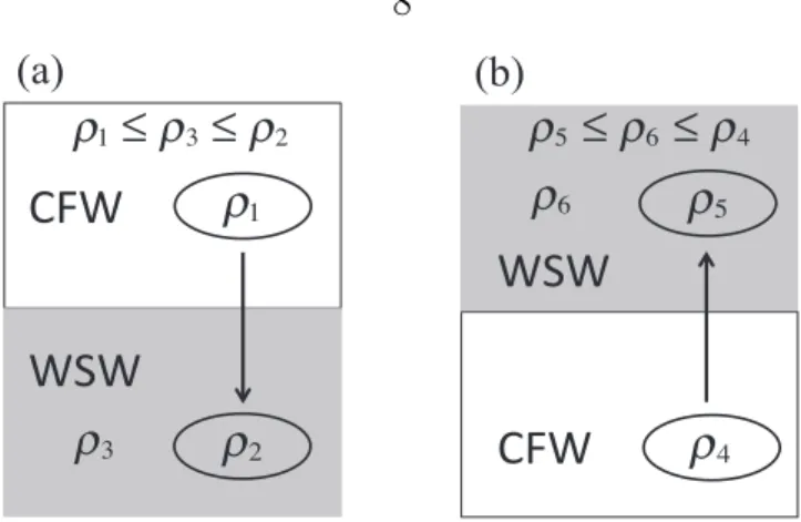
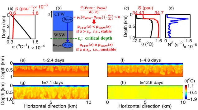
Here is a variable; the reference state by definition corresponds to adthat globally minimizes the PE of the state (1.13), where. Each possible reference state belongs to one of three cases, distinguishing between whether no CFW (Case 1), a fraction of the CFW (Case 2), or all the CFW (Case 3) moves below the WSW.
Case 2
Case 3
Alternative explanation for the threshold of Cases 1–3
Therefore, the initial column contains OCAPE, and the state of Reference corresponds to the value z, which makes zS = zc. Therefore, the initial column contains OCAPE, and the reference state corresponds to z = (1 )D (ie, all CFWs move below WSW).
Analytical expressions for OCAPE of more realistic profiles
The key point is that the PE difference between the current state and the rearrangement state is well approximated by the PE difference between the "transformed current state" and the "transformed rearrangement state"5. 5 In other words, the PE distinction between the current state and the "transformed current state".
Implications
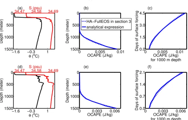
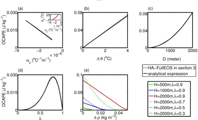
This is confirmed by the eight examples in Table 1.1, which shows the agreement between the analytically estimated OCAPE and the OCAPE calculated via HA-FullEOS (see also Section 1.6 for further verification using realistic profiles). Dashed and solid blue lines are from HA-FullEOS in Section 1.4 and analytical solutions derived from Section 1.5.4, respectively (see Section 1.6 for details). c) Estimated temporal evolution of OCAPE for 1000 m depth profiles in panel (a) during wintertime surface forced brine rejection.
OCAPE in the winter Weddell Sea
For an actual convection event, OCAPE based on the maximum depth of convection (⇠1000 m for this case) is the most dynamically appropriate. In Figure 1.4(d) we show another approximately two-layer profile from observations (McPhee et al., 1996).
Discussion and Conclusion
Key results
In this case, the dependence of OCAPE on the depth of the column (Figure 1.4(e)) and on the strength of the surface motion (Figure 1.4(f)) are similar to the previous example (Figure 1.4(b,c)). We quantitatively classify OCAPE in three different cases (section 1.5.2). v) We find an OCAPE J/kg from hydrographic profiles from the Weddell Sea in winter.
Limitations
Discussion
A possible example is the bilayer stratification in the winter Sea of Japan (see Figure 6 of Talley et al., 2004). The main diagnostic is ocean convective available potential energy (OCAPE), a concept introduced in Chapter 1.
Introduction
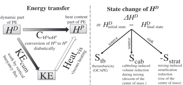
CHDtoHP, as described in section 2.5.3 and (2.15b), represents the time-integrated conversion from HD to HP due to diabatic processes. In Section 2.5 we increase the complexity of our simulation (using the full EOS) to evaluate and explain Scab and CHDtoHP.
Fundamentals for the energetics of Type II and Type III convection . 49
Numerical scheme
We calculatehP,hD and their derivatives (μP,CpP,μD andCpD) using the state functions of Jackett et al. To ensure numerical stability while minimally affecting turbulence, our standard vertical and horizontal viscosity and tracer diusivity are 3 ⇥10 4m2/s.
KE contributions from OCAPE and the reduction of stratification
Unstratified simulation without cabbeling
The sinks of OCAPE include Stb and Sinkdiab: Stb is the cumulative contribution of OCAPE to KE (Figure 2.1), while Sinkdiab is the cumulative dissipation of OCAPE by diabatic processes (defined in (2.18b)). In all simulations except those denoted as “x”, the flow is resolved without unphysical grid-scale KE accumulation.
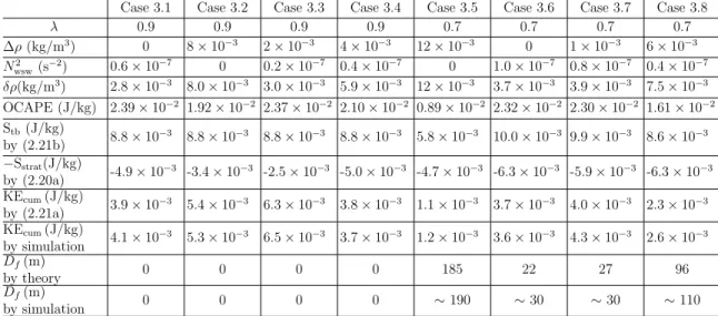
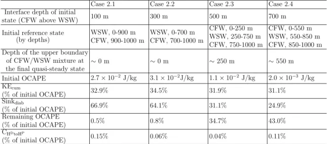
This ⇠1/3 conversion ratio from OCAPE to KEcum is essentially independent of the initial trigger (as long as the direct contribution to KE is small). The initial reference state is determined according to Part I. HiD (HfD) is expressed by (2.A10), with an unknown Df (the depth of the upper boundary of the CFW/WSW mixture in the final state; Figure 2.3(c)).
Contribution of reduced stratification to KE: S strat
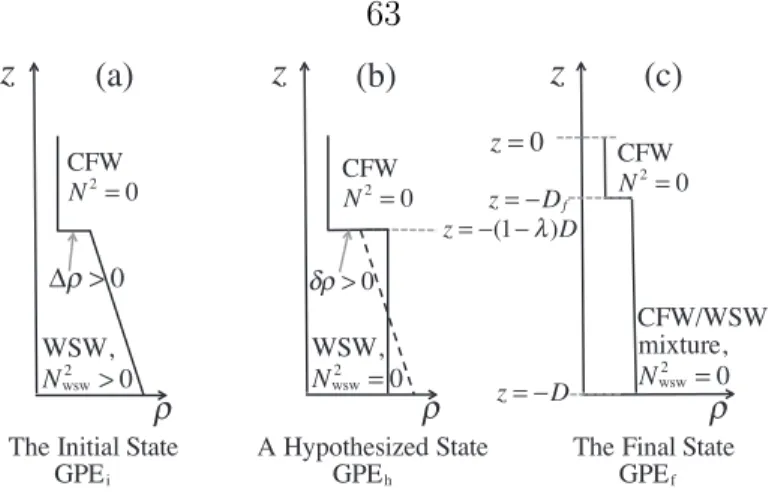
We also consider an assumed state (Figure 2.3(b)), the same as the initial state, except that the stratified WSW is replaced by the average WSW. Here OCAPec is the initial state OCAPE for the part of the water column where convection occurs3.
KE contributions from cabbeling-induced volume reduction and the
Unstratified simulation with cabbeling
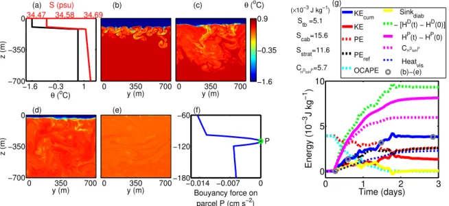
This comparison identifies important differences presented by cabling:. i) Convection initiation is faster (⇠ 0.22 days vs. 1.18 days) since the entrainment/mixing involved in the cable at the initial interface generates a negative motion and entrains the CFW plumes into the WSW faster. Panel (f) follows Figure 9(b) of Harcourt (2005) : it shows the buoyancy force on the P parcel using the full nonlinear EOS when it is shifted vertically and adiabatically along the initial profile.
KE contribution from cabbeling-induced volume reduction: S cab
The initial cooling applied to the simulation in Figure 2.2 is also applied to all simulations here. The initial cooling applied to the simulation in Figure 2.2 is also applied to all simulations here, triggering convection along with the wiring instability.
A theory to estimate the maximum depth of convection
For (g), see Figure 2.1 for detailed energy relations. iii) We assume that the final state is the one with the minimum PE, which is consistent with the simulations (see below) and the principle of least sum. Our predictions of convection depth with the above strategy are in close agreement with those found from numerical simulations (Figure 2.6(c)), which are diagnosed based on the maximum depth that convective clouds and subsequent mixing can reach.
Application to observed profiles
Discussion and Conclusion
Key results
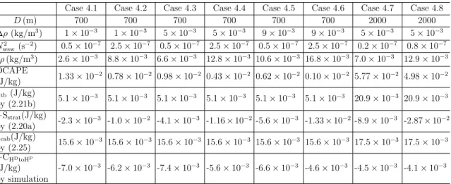
The fourth component is diagnosed numerically (table 2.4 and figure 2.6(b)). iii) Thermobarity (the first KE component above) dominates over cabbeling (the third KE component above) for deeper convection depths, while the latter dominates the former for shallower convection depths (Table 2.4, cases 4.1–4.6 vs. cases 4.7– 4.8). iv). We develop a theory to predict the maximum convection depth from the initial profile reproduced by the numerical simulations (Figure 2.6(c)).
Model limitations
Our choice to use 2D simulations reduces the computational burden and allows a greater exploration of the parameter space. It is possible that a more dynamic difference between these convection types can be identified from a buoyancy perspective (see Harcourt, 2005).
Implications
Mixing parameterizations in current ocean general circulation models (GCMs) typically use strong local diapycnal mixing in the vertical wherever the water column is statically unstable (e.g., KPP parameterization, Large et al., 1994). The parameterization for type II and type III convection, however, should include the vertical motion of ocean parcels to great depths without significant mixing at intermediate depths.
Appendix: Mathematical derivation of Equation (2.1)
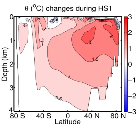
Then ⇢, the density difference between the CFW and the average WSW at the level of the CFW/WSW interface initially, has an expression. He etc. 2013) suggest that a warming of ⇠3–5oC occurred at intermediate depths in the North Atlantic over several millennia during Heinrich Stadial 1 (HS1), which caused warm saline water (WSW) to lie below the fresh water surface of cold.
Introduction
In this study (Su et al., 2016a) we propose a modified convective threshold mechanism, as a change to the above established convective threshold mechanism. Both modified and established convective threshold mechanisms are associated with the observed millennial-scale warming (⇠3-5 oC) in the intermediate depth (⇠1-2 km depth) of the North Atlantic during HS1 (Thiagarajan et al . 2014; Mar-cott et al. 2011; Alvarez-Solas et al. 2010).
Basin-scale OCAPE in the North Atlantic at the end of HS1
We use monthly CCSM3 simulation results of the last deglaciation (Liu et al. 2009; CCSM3 parameterizes vertical mixing due to internal wave breaking and other processes (Collins et al., 2006).
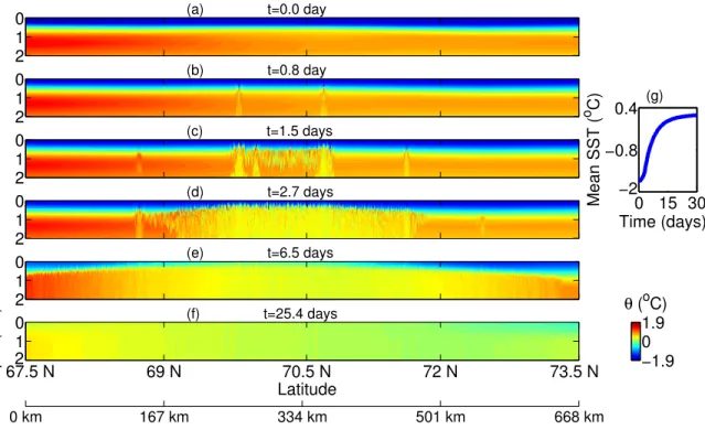
Simulated abrupt TCC events at the end of HS1
The simulation is initialized by the snapshot output ✓ and S from the CCSM3 simulation shown in Figure 3.3e. See Figure 3.5 for details of the convective plume and its lateral propagation (zooming to a local horizontal domain ⇠40 km).
Implications and further work
Martinson (1990) and McPhee (2003) demonstrate the major role of sea ice in maintaining the stability of the ocean columns. During convection, the warm water brought to the surface would melt the sea ice, thus re-moving the ocean column.
Introduction
Hieronymus and Nycander (2015, hereafter HN15) are the first to solve the Lorenz reference state exactly using the linear assignment algorithm (LAA, the so-called Hungarian algorithm). The Lorenz APE density is usually defined based on the Lorenz reference state and is a positive definite position function that integrates in Lorenz APE systems (Roullet and Klein 2009; Winters and Barkan 2013; see Tailleux 2013a for a review).
Solving the Lorenz Reference State
Our goal is to find the rearrangement state that has the absolute minimum PE (i.e., the Lorenz reference state). In essence, the Lorenz reference state is not unique: the redistribution of parcels along the corresponding pressure surfaces does not change the enthalpy/PE of the system.
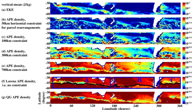
Eddy-size-constrained APE density
This black curve agrees well with the areas that have the smallest Lorenz APE density in Figure 4.2f (blue or green areas). The QG-APE of the World Ocean (Figure 4.6e vs 4.6d) has generally consistent patterns with the Lorenz APE.
Discussion
Figures 5a and 5b of Chen et al. 2014) shows the global map of the conversion term from eddy APE to EKE, and the conversion term from the mean APE to eddy APE, respectively, as diagnosed from the ECCO2 state estimate6. The QG-APE of a parcel is traditionally defined based on the deviation of density/buoyancy of this parcel from the horizontal mean of the considered system [e.g. equation (4) of Huang van Vallis 2006].
Introduction
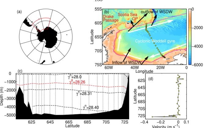
The magenta contour indicates the 1000 m isobath in the southern and western parts of the gyre. This approach is partly motivated by the striking isopycnal tilt seen in observations of the gyre boundary (Naveira Garabato et al., 2002).
An idealized Weddell Gyre
Bathymetry
At the northern edge of the roll, the 1 km isobath is discontinuous and we use a straight line to approximate the boundary. This produces a smooth representation of the bathymetry, but really captures the slope, especially around the edge of the roll (Figure 5.3).
Azimuthal winds
The components of the surface wind stress perpendicular to the 75 sections described in §5.3.1 are averaged to produce the azimuthal mean wind stress tangential to the gyre boundary. The relative amplitudes of the modes are the same at all radii from the gyre center.
Residual-mean dynamics
Since the azimuthal-mean isopycnal z =⌘(r, t) is a material surface in the sense of the residual advective derivative D†/Dt⌘@t+u†·r, it can be shown (see Appendix A) that it evolves according to. Equation (5.6) shows that the evolution of the isopycnal equilibrium must be compensated by the radial divergence of †, i.e.

The model solution
- Analytical solution in cylindrical basin
- Numerical solutions in a curved basin
- Sensitivity to wind stress and eddy di↵usivity
- Eddy suppression by the bathymetric slope
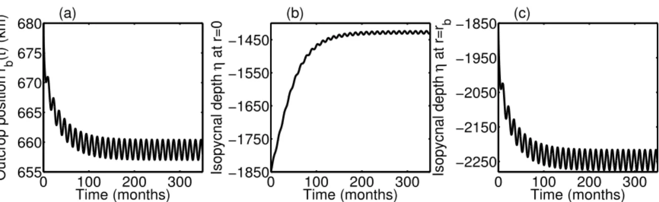
At the boundary of the eddy, the maximum isopycnal height lags (minimum) eleven (five) months behind the maximum wind load. Sensitivity to the eddy di↵diusivity , with fixed. a, e) The time-averaged isopycnal length⌘. b, f) Amplitude of the isopycnal oscillation|⌘0|.
The impact of inflow/outflow of WSDW
Parameterizing inflow/outflow of WSDW
Impact of WSDW inflow/outflow on the isopycnal oscillation . 158
Comparison with data
Model limitations
Model implications
Conclusion
Appendix A: The isopycnal evolution equation
Appendix B: Numerical scheme for a curved basin
Appendix C: Boundary current parameterization