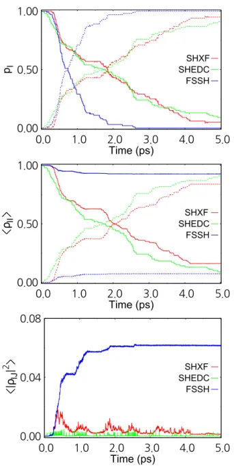
24 8 BO population (first and third row) and coherence profiles (second and fourth rows) for the SAC model with initial momentum k0 = 10.0 a.u. 42 9 BO population (first and third rows) and coherence profiles (second and fourth rows.) for the SAC model with initial momentum k0 = 25.0 a.u. 51 18 BO population (first and third row) and coherence profiles (second and fourth row .) for the DAG model with initial momentum k0 = 40.0 a.u.
Introduction
The resulting equations of motion contain the so-called "decoherence terms" which come from the coupled nuclear and electronic TDSEs from the exact factorization formalism. In this section, we first review the exact factorization formalism [ 64 , 65 ], the original FSSH and Ehrenfest dynamics, and derivation of MQC equations based on the exact factorization [ 31 , 32 ]. Then, we finally introduce the ITMQC-XF methods, which exploit the efficiency of the Ehrenfest and FSSH dynamics and correct ENC effect from the exact factorization formalism.
Exact factorization
The time evolution of the nuclear wave function is controlled by the time-dependent vector potential (TDVP). From the exact factorization of the nuclear and electronic wavefunctions (equation 9) and the PNC for the electronic wavefunction (equation 10), the nuclear and electronic wavefunctions are unique up to the following (R, t)-dependent gauge-like transformation . The nuclear wave function χ(R, t) defined in the exact factorization is the real nuclear wave function since χ(R, t) yields the exact many-body nuclear density and current density by definition.
Ehrenfest and fewest-switches surface hopping dynamics
Furthermore, the nuclear wavepacket never split in the Ehrenfest dynamics since the trajectory follows the mean potential. Since the nuclear trajectory is propagated by a certain BO force, FSSH dynamics can describe the exact separation of nuclear wave packets. If the nuclear trajectories cross the NAC regions many times, the internal consistency of the electronic dynamics can be broken, i.e.
Independent-trajectory mixed quantum-classical dynamics based on the
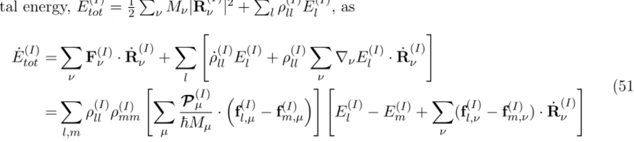
To calculate the decoherence terms, we need to calculate the nuclear quantum moment Pν and the phase term fl,ν. While the phase term can only be calculated from spatially local information on the position of the nuclear trajectory, the quantum momentum requires. Originally, the auxiliary trajectory propagates with the nuclear velocity (R˙(I)l,ν(t) = P(I)l,ν/Mν), which is determined by the total conservation of energy [22] as
Applications
In particular, after the last AC, the electronic state of the trajectory is decohered to the ground state, that is, for the FG width we fixed σ to the width of the Gaussian function for the initial nuclear wave function. Therefore, in the ECR model it is important to correctly capture both the nuclear dynamics and the electronic state evolution, as the ECR model includes the reflection of the nuclear wave function on the upper BO state.
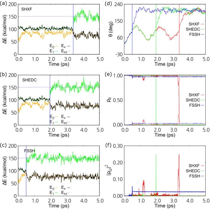
14 shows the time evolution of the BO population and the coherence for k0 = 26.0 au, where the reflection occurs on the upper BO state due to the insufficient nuclear kinetic energy. Because the upper and lower BO states are nearly degenerate at R < 0 au, the core wave packets are not separated and no subsequent decoherence occurs. The EhXF dynamics with the P phase cannot reproduce the correct reflection time or the second BO population transfer due to the total energy change, regardless of the auxiliary trajectory propagation or Gaussian width calculation methods.
After passing the NAC region at t≈600a.u., the nuclear wavepacket is partially transferred to the upper BO state in the exact dynamics. This is because some orbits are reflected onto the upper BO state due to the decrease in total energy. For the SAC model, all methods show small MAEs, which we expect due to the simplicity of the dynamics.
For the ECR model, due to the total energy change and incorrect nuclear dynamics, the EhXF dynamics with the P phase shows significantly large MAEs.
Conclusion
In particular, the EhXF dynamics with the A-EOM and P-phase show larger MAE than the original FSSH dynamics due to the incorrect reflection of trajectories. For the DAG model, the ITMQC-XF methods show significantly smaller MAEs than the original FSSH withσ = 20.0/k0. In particular, using the O-EOM in combination with the frozen Gaussian display significantly yields MAEs regardless of the phase term calculation method.
In terms of computational cost, the ITMQC-XF methods have almost the same computational cost as the original FSSH algorithm for the one-dimensional two-state model systems. Therefore, the SHXF dynamics with the A-EOM and EhXF dynamics will be computationally more expensive, because they also require nuclear gradients of "idle" potential energies of the BO state. However, for the extended systems such as molecular complexes and solids, one can use Ehrenfest dynamics in combination with real-time time-dependent density functional theory (RT-TDDFT).
In particular, the E phase is crucial for the EhXF dynamics to obtain correct simulation results. Therefore, SHXF-TD with O-EOM and the E phase will generally be an optimal choice. According to the benchmark test of different calculation methods for the elements necessary for the decoherence terms, we conclude that the SHXF method in combination with TD-width, E-phase and O-EOM is most promising in terms of accuracy and efficiency.
We conclude that EhXF combined with the E-phase can improve the Ehrenfest dynamics based on the RT-TDDFT formalism for various applications in materials chemistry.
Introduction
We present a new ML-ESMD strategy which trains diabatic Hamiltonian matrix elements based on SSR(2,2), i.e. we train three models for two diagonal elements and one off-diagonal element from direct minimization of loss functions with diabatic elements. Here we exploit phaseless loss function from the SchNarc approach [110] for training the off-diagonal element.
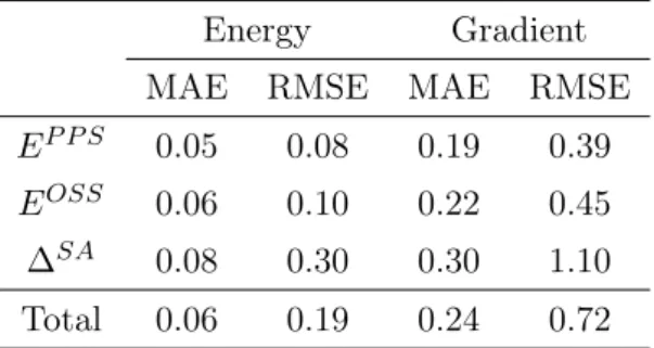
We show that reasonable accuracies can be obtained for the diabatic element Hamiltonians and their gradients with MAEs of ∼0.1 kcal/mol and ∼0.5 kcal/mol/Å, respectively, without any singularity problems for a specific ML with penta -2,4- dieniminium cation, a minimally protonated Schiff base (PSB3 for short). We also show that ML-ESMD for PSB3 provides a similar trend to a direct ESMD simulation. In addition, to check the transferability of our ML-ESMD scheme, we check the accuracy of the ML models with an extended training based on multiple species.
Method
Here, CLSA=wP P SCLP P S+wOSSCLOSS,nLpσinFˆσLare is the number of occupations of orbitalep with σ spin and the usual KS operator for the σ spin orbital of the Lth microstate, respectively np =P. Although SSR(2,2) is limited to computing only the lowest two singlet states, the general extension of SSR is quite straightforward. An SSR formulation suitable for describing the dissociation of multiple bonds is also available.
Like other active space methods, the availability of SSR is highly dependent on the choice of active spaces. Since all constituents for ESMD simulations can be calculated from these quantities, a direct ML-ESMD simulation is possible without any further approximation [121]. For training EP PS and EOSS, we use a squared loss, L2, for each EP PS and EOSS axis. 78) where EiM L and EiSSR represent the energy for the ith nuclear configuration of ML and SSR(2,2) approximations, respectively.
Ndata and Natom are the size of the training data set and the number of atoms in a given molecule, respectively. Thus, in this phase-free loss, the reference data with one of the two phase factors closest to the model is selected. After training the elements of the SSR(2,2) diabatic Hamiltonian, we calculate the BO quantities from equation 77 for direct ML-ESMD simulations.
To evaluate the validity of our ML-ESMD strategy, we first examine a PSB3, the well-known minimally protonated Schiff base, as a target system that has been extensively studied.
Application
A single point calculation with the resulting ML models including the diagonalization (~0.1 s) was about 1000 times faster than the SSR(2,2) calculation (~105s). Here we calculate a MECI and corresponding branch plane vectors of PSB3 from our ML models with penalty function algorithm [130] and we compare them with the SSR(2,2) method. Next, we explore the PESs around the CI in the branching space to check whether the ML models can capture the features of CIs.
The ability to reproduce the correct PES topology near the CI suggests that our ML models can replace the time-consuming quantum chemical calculation for ESMD. Finally, we perform ESMD simulations for PSB3 using the SHXF approach based on ML models (SHXF/ML). The evolution of the central dihedral angles C-C=C-C of randomly selected 50 trajectories during the dynamics is shown in comparison with the reference dynamics (Figure 26).
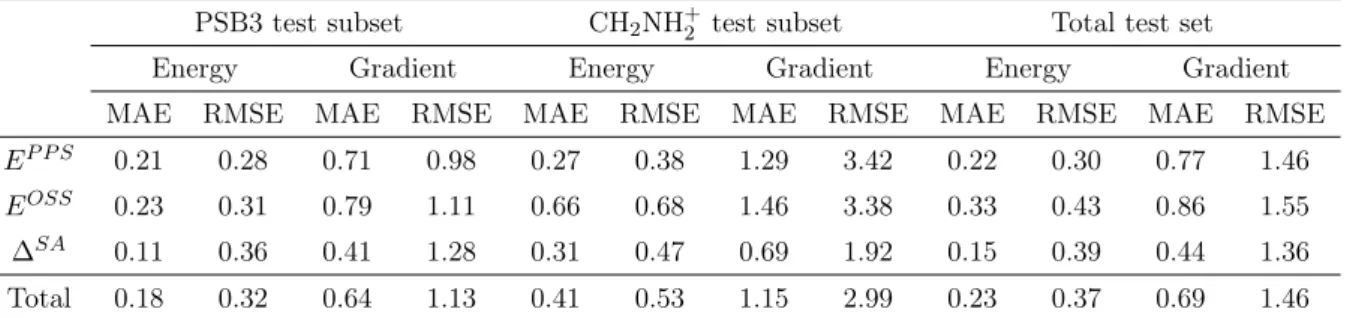
In this section, we train our ML models on an extended dataset consisting of two small protonated Schiff bases, PSB3 and CH2NH+2, to test the flexibility of the ML models in chemical space. We train the ML models with the extended training set of PSB3 and CH2NH+2 with the same training parameters used in the previous section. We estimate ML models on the PSB3 test subset, the CH2NH+2 test subset, and the entire test set.
The difference in error magnitudes between subsets indicates a biased fit of the ML models to PSB3, which originates from the relatively small size of the CH2NH+2 subset.
Conclusion
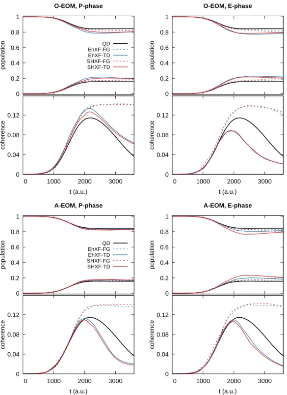
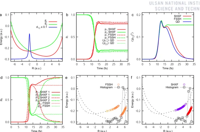
For the EhXF and SHXF dynamics, the solid and dashed lines represent the result for the TD and FG widths, respectively. The first and second columns represent the result for the P phase (equation 50) and the E phase (equation 53), respectively. The top and bottom four panels represent the results for O-EOM and A-EOM, respectively.
For the EhXF and SHXF dynamics, the empty and filled symbols represent the results for FG and TD widths, respectively. The first column presents the result for phase P (equation 50), while the second column presents the result for phase E (equation 53). The top four panels show the results for the O-EOM, and the bottom four panels show the results for the A-EOM.
The first column is the result for the P-phase (equation 50) while the second column is respectively for the E-phase (equation 53). The first row shows the results for the O-EOM and the second row shows the results for the A-EOM, respectively. Olivucci, "Tracing the excited-state time evolution of the visual pigment with multiconfigurational quantum chemistry,".
PES-Learn: An open source software package for the automated generation of machine learning models of molecular potential energy surfaces,” J. Jenkins, “Next generation quantum theory of atoms in molecules for the ground and excited state of DHCL,” Chem. I would like to thank Kicheol Kim for early work on machine learning-assisted molecular dynamics for excited states and technical assistance on computer hardware and software.