In chapter three, we examine the use of the phase vocoder for additive analysis-synthesis. We begin with a review of the phase vocoder and its relationship to short-time Fourier analysis. The new feature of our work is to explicitly relate the size of the phase vocoder and phase derived signals to the parameters of the additive model.
A proper understanding of a phase vocoder begins with an understanding of the time-dependent Fourier transform. Then e(n) = 0 and the magnitude of the phase vocoder is simply the magnitude of the true amplitude convolved with the impulse response h(n.
41- a. Input amplitude
43- a. Input amplitude
0 channel separation introduces severe distortions in the phase derivative signal for each filter; but distortions occur only at the minimum amplitude. First, this observation provides a useful perspective for examining the role of the phase vocoder in amplitude-independent pitch modification; let's return to this point for a moment. Finally, this observation is important if the phase vocoder is to be used with the additive model to study timbre; this is a major motivation for the phase-tracking vocoder of Section 3.7.
This also applies to the phase vocoder, provided the individual partials are well within their respective filter bandwidths. In contrast, it can be easily demonstrated that the frequency response of a system. which simply takes angle differences is. 3.47) , It follows that the angular difference is a good approximation to the phase derivative for small values of "'· An ideal integrator would have the frequency response. This is clearly the right thing to do for the angular differences, but not for the phase derivative except for small values of GJ.
Since typical music and speech signals include fairly large values of GJ, the use of the phase derivative is inevitably a source of error. The first of these is to use the angular differences in place of the phase-derived signal, and to reconstruct the phase by simple addition. On reflection, this seems reasonable because the transformation of equation (3.50) is precisely the one that keeps the phase-derived signals of Figures 11b and 12b properly synchronized.
The phase vocoder makes the tacit assumption that the signal in each filter channel (at least over a suitable time period) is a pure sine wave.
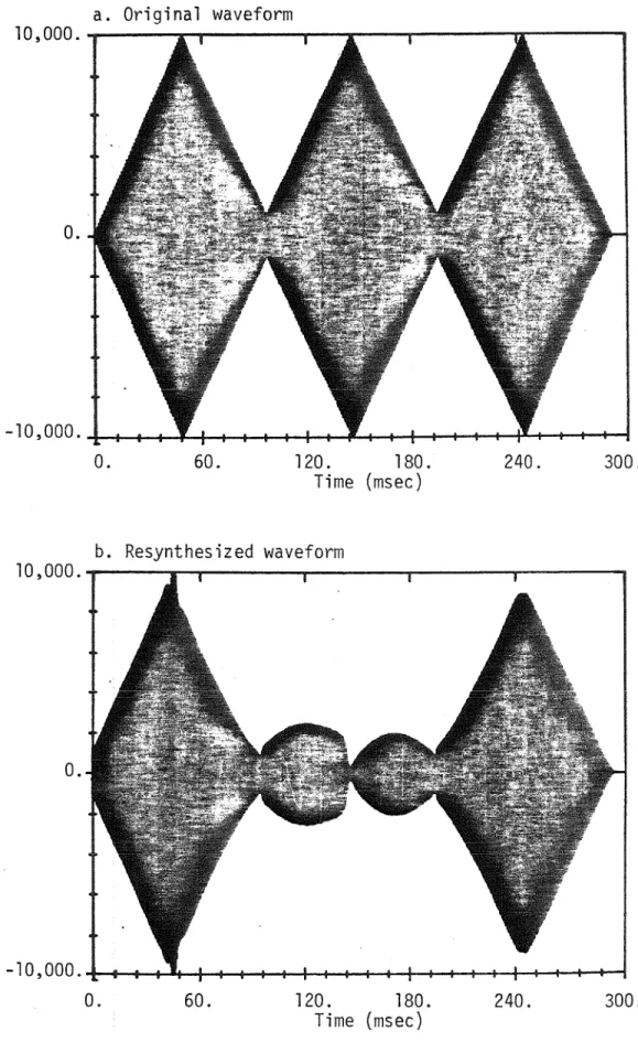
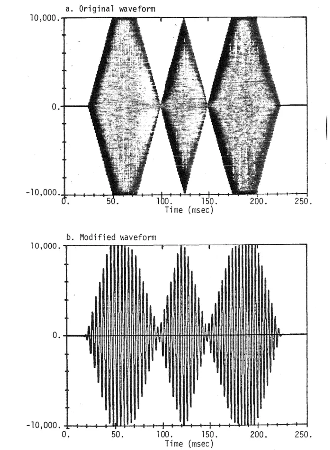
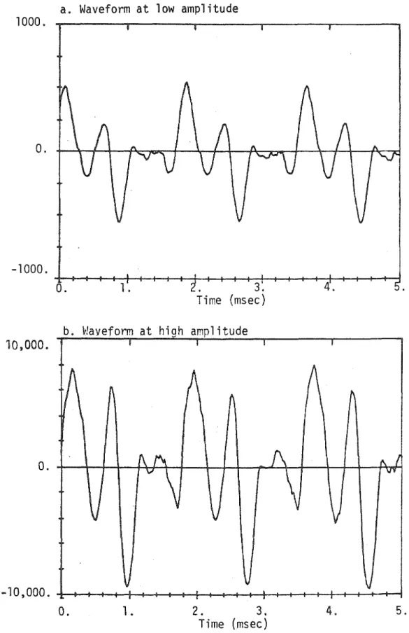
51- a. Original waveform
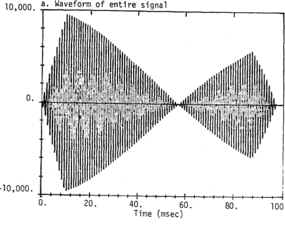
Alternatively, we can simply view the signal-plus-noise case as a subset of the case that follows. 1s shows that the instantaneous frequency of the sum is the average of the instantaneous frequencies except for occasional spikes due to the phase change showing that a small sine wave imposes a simultaneous amplitude and frequency modulation to a larger sine wave occupying the same channel . In both cases, it is clear that the phase-derived peak is simply an artifact of the analysis technique; a narrowband filter centered on the peak frequency of the peak will not detect any energy at any time.
Therefore, we conclude that phase curves within a given phase vocoder channel are not perceptually relevant. As a result, voice modifications of the type defined by equation (3.23) can have undesirable effects on timbre. Finally, we consider an extension of the above analysis, which is important for Chapter 4 to follow.
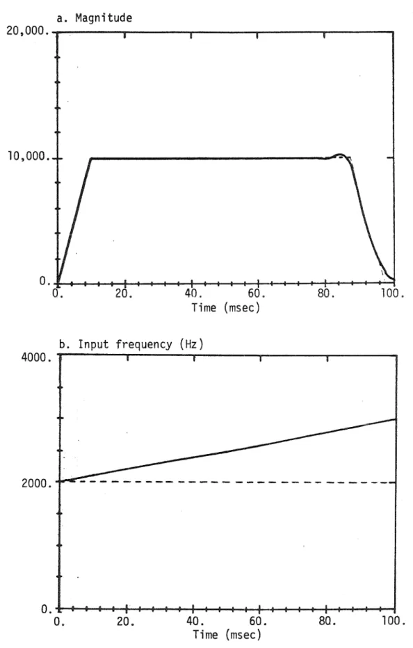
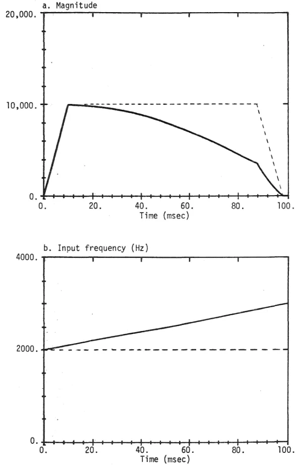
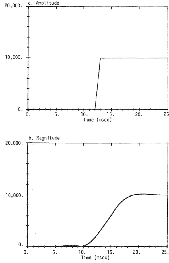
Moorer [1978] reported that the non-band nature of the magnitude and phase conversion made it necessary to calculate these signals on the. If the instantaneous frequency is not centered within the filter bandpass, a rapid change in frequency can significantly increase the bandwidth of the magnitude signal; but this is rare. An important example of this banding is given in Figure 17, where the response of the magnitude signal to a step change in amplitude is found to be almost equal to the step response of the filter.
Consequently, we are forced to numerically determine the bandwidth of the magnitude signal for some representative cases.
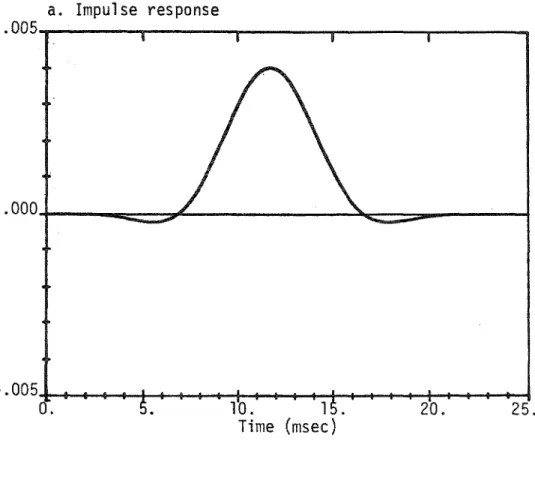
61- a. Impulse response
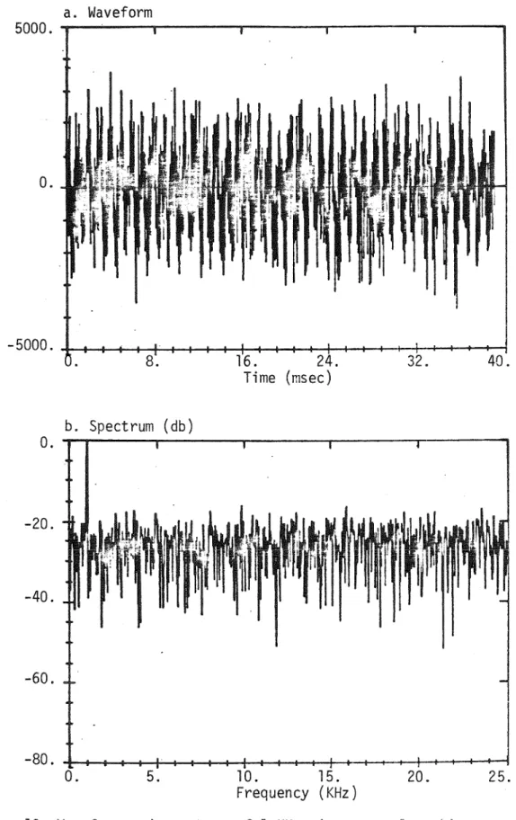
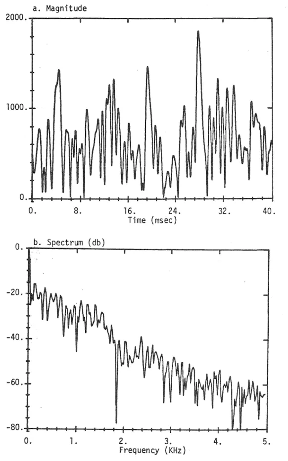
This provides a means to realistically study narrowband signals and at the same time compare the effects of different filters, which cannot always be implemented with narrow bandwidths. To determine the approximate bandwidth of the magnitude signal, we use a 3‐term Blackman‐Harris window [ Harris , 1978 ] and take a 2048‐point fast Fourier transform using zero padding where appropriate. The spectrum in Fig. 19b clearly shows that the magnitude signal is still effectively band-limited by the filter in this case.
Indeed, we consistently found this case to be the one in which the magnitude signal reached its maximum bandwidth. The exact value of this bandwidth depends on which definition is adopted, but we observed two consistent trends. First, the spectrum of the magnitude signal depended surprisingly little on the sharpness of the filter cutoff: this is shown in Figures 21 and 22 for the 2000 Hz center frequency and the two filters in Figure 5 .
Second, the bandwidth of the magnitude signal (as measured at the -40 db point) was usually less than the channel separation. We did not test the perceptual effects of undersampling, but we suspect that such effects would be least apparent precisely in those cases where the magnitude signal achieves its greatest bandwidth - ie.
67- a. Magnitude
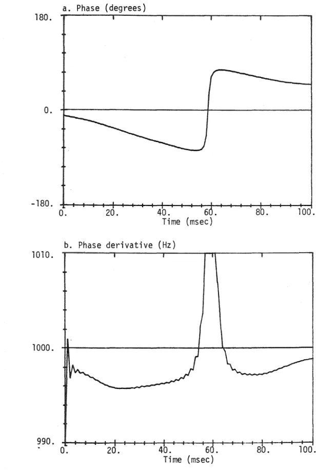
We first examine the response of the phase derivative signal to a step change in frequency (assuming that both the initial and final frequencies are well within the filter bandpass). First we note that, in the absence of points, the bandwidth of the phase derivative signal is significantly smaller. Conceptually, a pitch-tracking phase vocoder is a simple extension of the standard phase vocoder described in previous sections.
In this section we summarize these advantages and show how a tracking version of the phase vocoder can be easily implemented. It is more complex to implement, but its accuracy (in terms of resynthesis) can never exceed that of the standard phase vocoder. However, even with this precaution, the ultimate performance depends on the intelligence of the tracking algorithm.
An example of the phase tracking vocoder output is given in Figure 28 for the input signal in Figure 13a. However, the re-synthesized signal is actually worse than the stationary phase vocoder signal (which is perfect) due to the band-limiting of the magnitude signal in the tracking version. Instead, it is better than the phase signal. because it allows accurate phase reconstruction.
A third (and unanticipated) limitation was the quality of sound examples available to us.
91- a. Amplitude
In this representation, we sought to capture average values rather than modulation details. This is illustrated for the amplitudes of the first eight parts of a typical tone in Figure 33.). We also found that each modulation produced a large improvement in realism, but that both amplitude and frequency modulation were necessary for the final effect.
We also used our enhanced analysis capabilities to examine the harmony of the violin parts. Line segment approximation for the amplitude of the first eight parts of a tone played with vibrato. We found that the violin parts were, in fact, harmonious, except perhaps during the attacking part of the tone.
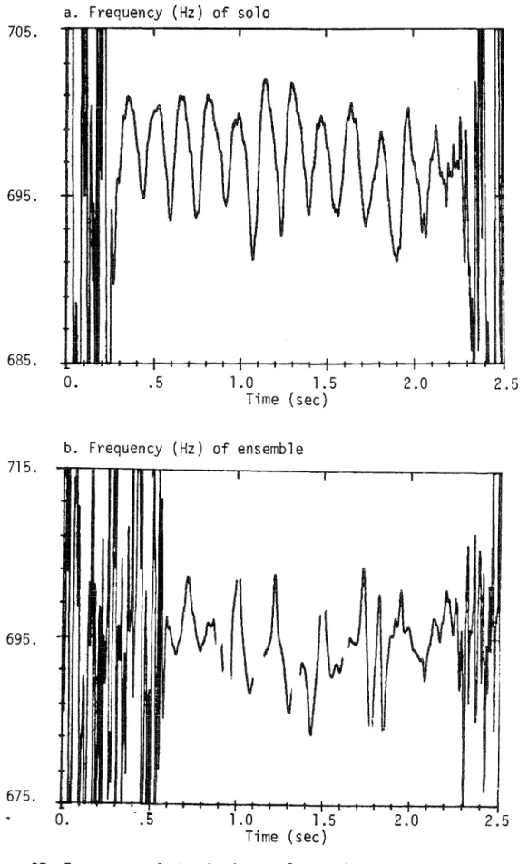
Since ensemble sound arises from different instruments playing simultaneously, we also analyzed several different violins individually to determine the extent of the variations between them. But for the violin it is more appropriate to take a dynamic view, where each reflection has its own particular pitch corresponding to the particular phase of the vibrato cycle in which it arose. Another obvious difference between solo and ensemble can be seen in figures 37 and 39; the composite frequency of the four violins shows almost no trace of the individual vibratos.
Indeed, for higher harmonics, it is difficult to make any sense at all of the frequency estimates provided by the phase vocoder.
97- a. Wavefonn of solo
99- a. Amplitude of solo
Therefore, we concluded that ensemble amplitude variation was sufficient but not absolutely necessary for ensemble sensation. We first asked whether a certain part of the tone itself was sufficient to produce an ensemble feeling. We therefore wondered whether the steady state part of the ensemble would still be identifiable as an ensemble.
This is an indication that the room reverberation introduces a significant overlap of the two tones. Furthermore, we know very little about the detailed interactions between the musicians in the context of the ensemble. In general, we found that the faster beat of the higher sections in the actual ensemble was essential to prevent the ear.
On the other hand, the fast beating of the lower parts just made the ensemble sound bad. Another aspect of the ensemble feel that we tried to investigate was the number of instruments in the ensemble. As a result, the decisive factor in the sound of the ensemble was not the number of solos, but the relative phase of the vibrato in the individual solos.
For amplitude modulation, this variation is a beat proportional to the average frequency of the partial signal.
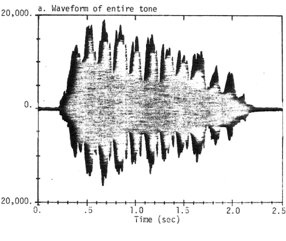
2.0 Figure 48. Amplitude and frequency of the fundamental of the
Ar.fib, D., "Digital Synthesis of Complex Spectra by Multiplying Nonlinear Distorted Sine Waves," J. Jnternational Conference on Acoustics, Speech, and Signal Processing, Atlanta, Georgia, March 2B - April 1 (19B1 ) Le Brun, M., "Digital Waveshaping Synthesis," J. Malah, D., "Time-domain Algorithms for Harmonic Bandwidth Reduction and Time Scaling of Speech Signals," lE.E.E.
McAdams, S., "The effect of spectral fusion on pitch perception for complex tones", Summary in J. Portnoff, M.R., "Time-frequency representation of digital signals and systems based on short-term Fourier analysis", J.E.E.E. Rabiner, L.R., and Gold, B., Theory and Application of Digital Signal Processing, Prentice-Hall, Englewood Cliffs, New Jersey (1975).
Schafer, R.W., and Rabine:r, L.R., "Design and Simulation of a Speech Analysis System - A Synthesis Based on Short Time Fourier Analysis," JE.E.E.