The integration of bank syndicated loan and junk bond markets

(1)

The integration of bank syndicated loan and junk bond markets

Hugh Thomas

^a,*

, Zhiqiang Wang

^b

aDepartment of Finance, The Chinese University of Hong Kong, Shatin, NT, Hong Kong SAR, China

bDongbei University of Finance & Economics, Dalian, Liaoning, China

Accepted 13 January 2003

Abstract

This paper hypothesizes that the special role of banks as corporate quasi-insiders has been changing due to developments in informational, legal and institutional infrastructures of syndicated loan markets. We investigate the integration of intermediated and disintermediated ﬁnancial markets through highly leveraged transaction (HLT) syndicated loans during the 1990s. We demonstrate that, with the emergence of traded HLT syndicated loans as an alter- native high-yield asset to high-yield bonds, market integration has dramatically increased.

Taking the late 1980s and 1990s together, diﬀerent factors explain the movement of credit spreads of the two markets. HLT loan market’s spreads are strongly aﬀected by bank liquidity.

Bank liquidity’s eﬀect on HLT loan spreads disappears after 1993. From 1994–1999, junk bond market liquidity factors aﬀect bank loan pricing. We interpret these changes as evidence of the erosion of bank specialness.

JEL classiﬁcation:G14; G21

Keywords:Syndicated loans; Junk bonds; Disintermediation; Credit spreads; Bank loan pricing; Bank liquidity; Special role of banks; High yield bonds; Highly leveraged transactions

1. Introduction

The banking literature commonly characterizes loans as illiquid assets. The lender is assumed to possess relationship-speciﬁc skills and/or information that preclude the

*Corresponding author. Tel.: +852-26097440; fax: +852-26035136.

E-mailaddress:[email protected](H. Thomas).

doi:10.1016/j.jbankﬁn.2003.01.001

www.elsevier.com/locate/econbase

(2)

efficient trading of loans in secondary markets where they would compete with public securities. This characterization helps us to understand the nature of banking, yet it is a simplification of reality. Loans have never been absolutely illiquid. Correspon- dent banks traditionally have been able to effect portfolio re-balancing by exchang- ing assets as long as the relationship between buyer and seller was strong enough to generate sufficient trust to mitigate informational asymmetries between them. Loan sales by bankruptcy trustees have long been a part of winding up failed banks. The marketability of bank loans, then, is a question of degree. Today, that degree is rapidly increasing.

Banking is an information industry so it is not surprising that the 1990s revolution in information technology fundamentally aﬀected banking. At the strategic level, leaders of the top banks around the world are unanimous that their models of business are undergoing substantial change.¹Secondary market loan trading has also developed radically. Legal changes set the stage for standardization of loan trading and a rapid rise in trading volumes. The Loan Syndication and Trading Association has been set up to facilitate this process. Bond rating agencies are now rating syndicated loans.

Given these changes, the ﬁnancial academic’s question, ‘‘why are banks special?’’

perhaps should be rephrased. In a recent article, Bossone (2001) asks, ‘‘Are transaction costs and information asymmetries being so dramatically reduced in modern ﬁnancial systems that what was once special about issuing liquid liabilities and ﬁnancing illiquid assets is hardly special at all, today?’’ Bossone answers his question from his theoretical analysis in the negative.

We hypothesize that the special role of banks as corporate quasi-insiders has been changing due to developments in informational, legal and institutional infrastructures of syndicated loan markets. We take an empirical approach, focusing on one banking service: syndicated lending. We ask the question, ‘‘are syndicated loans special and, if they are, is that specialness being eroded?’’ We answer this question by examining the degree to which the pricing of loans that are traded on the secondary market is integrated with the pricing of bonds.

We study highly leveraged transaction syndicated loans (HLTs) ²and compare their pricing to the pricing of high-yield bonds from January 1987 to December 1999. We build on the work of Angbazo et al. (1998) by estimating a model of the promised spread of HLTs above treasuries and comparing it to an estimated model of the yield spread of high-yield bonds above treasuries. We describe how the degree

1See Engler and Essinger (2000) who report wide-ranging interviews with the leaders Bank of Tokyo- Mitsubishi, Banco Santander, Central Hispano, Chase, Citigroup, Deutsche Bank, Goldman Sachs Mediobanca, Merrill Lynch, Morgan Stanley Dean Witter, Paribas, Societe Generale, etc.

2The term ‘‘HLT’’ refers to loans to borrowers whose senior debt is non-investment grade and whose loans are priced in excess of 225 basis points above LIBOR orwhose loan is to be used in a highly leveraged transaction such as a leveraged buyout. Although HLTs are not necessarily syndicated, only those that are syndicated have their terms and conditions widely reported. Hence, all of the HLTs we refer to in this paper are syndicated; moreover, when we refer to HLTs in this paper, we refer only to highly leveraged transactionsyndicatedloans.

(3)

of segmentation between bank and bond markets has been severely eroded over the last decade. We show that from 1987 to 1993 an excess (lack) of liquidity in bank markets leads to price falls (rises) in HLT spreads but that this effect disappears from the period 1994–1999. We show that bond market liquidity has no independent effect on HLT pricing in the earlier period but that in the later period increases (decreases) in junk bond market liquidity lead to increases (decreases) in HLT spreads. In summary, we find strong evidence that, in this important part of the lending market, bank specialness is indeed changing.

Our article is organized as follows. A brief introduction to the HLT market is found in Section 2. Section 3 is a review the literature on the specialness of banking and its relationship to syndicated lending. Sections 4–6 discuss our approach to measuring market integration, the data and our findings respectively. Section 7 concludes with a summary, a note concerning the degree to which our findings can be general- ized to other banking services, a comment on similar findings in related studies and some suggestions for further research.

2. The highly leveraged transaction syndicated loan market

Syndicated loans – loans that, prior to signing, are shared among groups of banks – have long been a part of corporate ﬁnance. A syndicated loan has traditionally allowed a lead bank³to arrange a loan so large that the bank, acting alone, could not book it without either breaching prudent concentration limits or reducing unacceptably its ability to do further business with the borrower, the borrower’s industry, and/or the borrower’s country. Through syndication, a lead bank can increase its return on risk capital from arrangement fee income while participant banks⁴can obtain exposure otherwise not available.

A syndicated loan is usually initiated by an underwritten oﬀer from the lead bank.

The oﬀer lists the borrower, underwriters, availability, tenor, interest rate, commit- ment fees, management fee, agency fees, syndication plan, security, covenants, etc.

but is subject to negotiation of the loan agreement which is signed by all lenders, each of which legally acts independently and individually to make the loan. Once the borrower has accepted an underwritten oﬀer, the underwriter(s)/lead manager(s) invites other prospective borrowers, outlining the transaction and the borrower’s sta- tus in an information memorandum. The loan agreement itself is actually signed by

3We use the term ‘‘lead bank’’ to mean the bankor banksthat initiate(s), underwrite(s) and arrange(s) the syndication transaction. This is typically the bank(s) having a strong relationship with the borrower.

We use the term ‘‘banks’’ loosely to include commercial and investment banks as well as other wholesale ﬁnancial institutions participating in the syndicated loans market.

4We use the term ‘‘participant bank’’ to mean the banks in the syndication that do not have a primary role in underwriting, negotiating, syndicating and otherwise arranging the loan (and obtaining fees therefrom) but enter the transaction with the purpose of booking a loan asset. These participants may be labeled as ‘‘co-lead managers’’, ‘‘managers’’ ‘‘co-managers’’, etc., but these names tend to be honoriﬁc, with higher sounding titles given to FIs that take larger shares of the loan.

(4)

each lender, and loan drawdown does not occur until after loan signing and clearing of legal conditions precedent to drawdown. The agent for the lenders liaises between the borrower and the lenders throughout the life of the loan. It arranges for clearing conditions precedent, receiving notiﬁcations for drawdown from the borrower and passing them to the lenders, channeling funds of drawdown and repayment, calculating interest payable, and distributing borrower information.

Lending banks tend to book syndicated loans to maturity, yet lead banks have long recognized the advantage of increasing syndicated loan secondary market liquidity. A more liquid instrument requires from lenders a lower liquidity premium.

Borrowers and lenders share the beneﬁts from improved loan pricing. Legal devices and increased informational transparency increase liquidity. Loan documentation typically contemplates loan sales, providing for assignment of loan participation. ⁵ Information availability facilitates secondary market liquidity: the lead bank for- mally places a large amount of borrower and facility information in the information memorandum for distribution to prospective lenders during syndication. Informa- tion is subsequently updated by borrower communication with the syndicate banks through the bank acting as agent for the lenders. Although not publicly available, these data can be easily and credibly forwarded to interested prospective purchasers in the secondary market. These liquidity-enhancing devices are not new, but the emergence of a true secondary market in syndicated loans is.

Fig. 1 shows that the volume of trading of syndicated loans on the secondary market rose from $8 billion (of mostly distressed debt) per year in 1991 to $110 billion (of mostly par loans) in 2001.⁶As we demonstrate below, this rapid increase in trading coincided with a change in the basis of pricing syndicated loans from a bank liquidity orientation to a capital markets orientation. Market, regulatory, legal and informational factors combined to stimulate this transformation.⁷

In the mid to late 1980s, the most active component of the secondary market for syndicated loan participations was less developed country (LDC) debt. During the LDC debt crisis, at one time or another, virtually all LDC debt became distressed,

5In this discussion, we refer to true sales of loans without recourse. Credit riskcanbe off-laid with risk participations (funded or unfunded) and with various credit derivatives. In such cases, the party that originally booked the loan maintains legally the rights and obligations of the loan but contracts with a third party to off-lay some portion of the risk and/or funding. In a sale by assignment, the sold loan is removed from the seller’s balance sheet and the seller has no liability if the loan defaults (unless the buyer can prove seller misrepresentation). Assignments typically require borrower agreement (or at least notification). Loan agreements structured to increase secondary market liquidity frequently contain clauses such that the assignor lender, by simple notice to the agent, legally causes the creation of a new loan (‘‘novation’’ of the contract) where all parties have the same rights and obligations but the assignee lender is substituted for the assignor. For the LSTA’s model assignment agreement, see http://

www.lsta.org/.

6‘‘Distressed debt’’ refers to loans that trade for less than 90 cents to the dollar of principal amount.

‘‘Par loans’’ are those that trade at more than 90 cents to the dollar. In 2001 distressed debt trading increased dramatically with the recession.

7Fabozzi (1998) has edited a collection of 11 essays by syndications market bankers that describe many of the developments summarized below.

(5)

but fair values varied greatly by country and issue, and were subject to dramatic changes over time. These events created an opportunity for proﬁtable trading.

Strategic rethinking by lending banks – sometimes under regulatory pressure – led many to exit the LDC debt market providing a supply of LDC debt to the secondary market. The market’s intermediaries were globally active commercial and investment banks, but most ultimate buyers and sellers were commercial banks with international portfolios. The market merely increased the scale of existing practices of the international syndications market. The assets’ bid-ask spreads were large – being several percentage points – and the market was illiquid relative to securities markets.

HLT syndicated lending was born in the late 1980s US merger boom and provided the assets that eventually extended syndications secondary markets beyond banks. Often a bridging vehicle in corporate mergers and acquisitions, HLT loans provided massive, rapid and ﬂexible ﬁnancing for leveraged buyouts. The HLT boom led to improvements in disbursement of syndicated lending information. Syn- dicated lending information is quasi-public: lead managers must distribute at least the summary terms and conditions and often the whole information memorandum to a relatively wide market in order to sell down the transaction. In 1987, Loan Pric- ing Corporation initiated itsGold Sheetsthat set out in a standardized form primary market information and distributed that information to paying subscribers.⁸

Par = total volume in billions of dollars per annum of loans that are traded at a purchase price of more than 90 cents per dollar of face value.

Distressed = total volume in billions of dollars per annum of loans that are traded at a purchase price of less than 90 cents per dollar of face value.

Total Activity = Par + Distressed.

Source: Loan Pricing Corporation 0

20 40 60 80 100 120 140

1991 1992 1993 1994 1995 1996 1997 1998 1999 2000 2001 year

billions of dollars

Par Distressed Total Activity

Fig. 1. Secondary loan market trading volume.

8TheGold Sheetswere not the first syndicated loan information service. In the 1970s,Agefiwhich in the 1980s becameInternationalFinancing Reviewprovided information on offshore Eurobanking syndicated credits. IFR is now owned by Thomson and provides global capital markets and syndicated banking information in competition with LPC, who is currently owed by Reuters.

(6)

In 1990, a legal change occurred that allowed the secondary market for syndicated loans to extend beyond banks. Loans are securities. If they were deemed to bepub- licly traded securities, they would be governed in the US by the Securities Act of 1933. The stringent requirements of that act eﬀectively limited the degree to which bank loans could be traded prior to 1990. In 1990, Rule 144A was passed allowing participations in syndicated loans to trade in a lightly regulated institutional investor market.

With the legal basis for broadened trading in syndicated loan participations in place, the credit crunch of 1991–1992 provided a supply of secondary HLT paper as some previously lending banks scrambled to rebalance their portfolios. Five investment and commercial banks rose to the opportunity to make a market in the outstanding loans, bringing liquidity to the market.⁹Some of these assets were distressed, but many were not. In 1994, for the ﬁrst time, the volume of par value loans traded in the market exceeded the volume of distressed loans. In 1995, two key events indicated that participations in syndicated loans might legitimately be called a capital markets asset class in their own right. First the Loan Syndication and Trading Association was founded to develop the market for the assets and sec- ondly, the bond ratings agency Standard and Poor’s initiated its program to rate corporate syndicated loans. Moody’s followed suit shortly thereafter. Table 1 provides a summary of factors that promoted the rapid rise of the secondary market for participations in syndicated loans.¹⁰

Unlike the market in loans prior to the 1990s, when commercial banks formed the main purchasers of loans, institutional investors accounted for most of secondary market demand during the 1990s. The market has gone beyond its banking roots.

Syndicated loans provide to institutional investors higher returns than traditional bonds. Yet institutional investors typically need spreads of 175 basis points over LIBOR to attract them into these non-traditional assets. That higher return is available in HLTs. Hence it is not surprising that, although HLTs account for a minority of the total amount of syndicated loans outstanding, they account for more than 80% of secondary market trading.¹¹This dominance makes HLT pricing an important and accessible area of study.

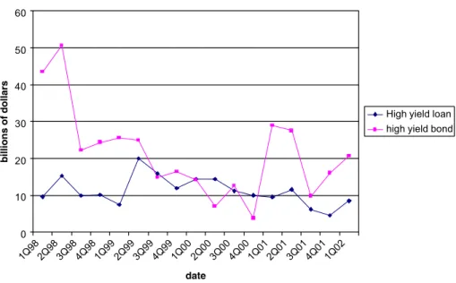
HLTs are also of interest for another reason. They have a parallel publicly traded security: non-investment grade (also called ‘‘high yield’’ or ‘‘junk’’) bonds. More- over, as Fig. 2 shows, the volumes of HLT issuance is of the same order of magnitude as junk bond issuance.

9Those ﬁrst making a market were BT Alex Brown, Bear Stearns, Citibank, Continental Bank, and Goldman Sachs (see Miller, 1997).

10For more information on this history see Bavaria (1998), Fabozzi (1998), the Loan Syndication and Trading Association website, Loan Pricing Corporation and Taylor (2000).

11Loan Pricing Corporation reports that in 2001, of the $159 billion in secondary market trades of par loans, only $27 billion were for investment grade (i.e., rated BBB and above) loans. Note, however, that HLTs account for only about 20% of total volume of new global syndications: in 2001, total global syndications were about $1.1 trillion while HLT syndications were $218 billion (Coﬀey, 2002). We return to this point in the concluding discussion of the implications of our study.

(7)

The above discussion has highlighted several aspects of the HLT market. It emerged from a traditional banking activity. Through time and owing to institutional, legal and informational reform, the volume of HLT trading has increased substantially. We hypothesize that HLTs have changed: they were a special bank service, but they are now priced in the wider capital markets. The existence of a parallel junk bond market serving the same borrowers allows us to test this hypothesis. But before we describe the tests and their results, we review brieﬂy the literature on bank specialness in lending.

3. Bank specialness and syndicated loan sales

A dominant theme in the banking literature is the role of banks in funding projects characterized by informational asymmetries and moral hazard. If banks are truly unique in their solution to these problems, we are left in a quandary: how do we to explain a growing market selling HLTs to non-banks?

Table 1

Events promoting secondary trading in the syndicated loan market

Date Event Signiﬁcance to syndicated loan secondary

market development 1985–1989 HLT syndicated lending powers merger

boom

HLT syndicated loans emerge as a major commercial bank asset class

1987 Loan Pricing Corporation starts publication of gold sheets

Standardized data on syndicated loan pricing published

1990 Rule 144A – private re-sales of securities to institutions amendment to the Securi- ties Act of 1933 passed by US Congress to allow companies to issue exempt securities for institutional investor market

Legal basis for institutional investor secondary market for syndicated loans established

1991–1992 Loan default rates on syndicated loans increase during recession credit crunch

Bank demands to exit markets through loan sales stimulates ﬁve banks to set up secondary loan trading desks

1994 Volume of par value loans traded in secondary market exceeds volume of distressed loans

Portfolio re-balancing of viable asset class of ongoing exposures becomes dominant 1995 Loan Syndication and Trading Associa-

tion founded and T + 10 convention adopted for par loans

Establishes organization to promote development trading market for corporate loans; standardizes conﬁrmation and settlement procedures

1995 Introduction of bank loan ratings by Standard and Poor’s

Establishes instrument-speciﬁc rating 1998 LSTA code of conduct published Promotion of integrity, fairness, eﬃciency

and liquidity through adoption of common standards

2002 CUSIP group of LSTA and Standard and Poor’s establish unique identiﬁer for each syndicated loan

Standardization will facilitate identiﬁca- tion among market participants analysis by researchers

Sources:LSTA, LPC, Fabozzi (1998).

(8)

Diamond’s (1984) banks function as delegated monitors, contracting with depositors to pay a fixed return based on portfolio diversification of project risk. HLTs seem to fit Diamond’s projects: they are large (relative to investors) and risky (as evidenced by their spreads). As Freixas and Rochet (1997) point out, delegated monitoring in Diamond’s sense need not take place in a banking environment. Banks comparative advantage is based on ingredients including scale economies in monitoring, small capacity of investors relative to projects and low costs of delegation. At first glance, the coalition structure of a syndicated loan might even be considered delegated monitoring. In Section 2, we described the role of the agent for the lenders in a loan syndication. The delegation of authority to the agent for the lenders, however, is clearly not delegated monitoring in a Diamond (1984) sense. The agent for the lenders in a syndication performs a relatively mechanical role, almost devoid of discretion. Asset management – particularly the decision to declare the occurrence of an event of default – is in the hands of the participant lenders. The agent bank in the syndication is only a nexus of information and cash flows, with very little discretion.

As we discussed above, institutional investors are increasingly lenders in HLTs.

Either these new lenders are forgoing monitoring (and thereby free-riding), or information transparency has progressed for this class of investors to allow monitoring without the lender itself being a quasi-insider-monitor.

In a dynamic context, Sharp (1990) and Rajan (1992) modiﬁed Diamond’s conclusions to allow for borrower reputation. Borrowers who can build reputation can ac-

High yield loan = total value of new principal of HLT syndicated loans issued in the quarter High yield bond = total value of new junk bonds issued in the quarter

Source: Loan Pricing Corporation 0

10 20 30 40 50 60

1Q98 2Q98 3Q98 4Q98 1Q99 2Q99 3Q99 4Q99 1Q00 2Q00 3Q00 4Q00 1Q01 2Q01 3Q01 4Q01 1Q02 date

billions of dollars

High yield loan high yield bond

Fig. 2. Junk bond versus HLT loan issuance.

(9)

cess public markets, avoiding the more expensive intermediated markets. These models more richly model the interplay between disintermediated and intermediated markets. Diamond (1997) demonstrates the role of banks coexisting with public markets due to the limited participation of some investors in the public markets. An implica- tion of his work is that, as direct participation by more investors in the public markets increases, so does disintermediation. Market demand-driven disintermediation directs more funds towards institutional investors. As noted above, the institutional investors are precisely the net buyers in the secondary markets for HLTs studied by us. In an international cross-sectional study, Buch (2002) documents that the ratio of bank lending to total cross border debt (bank lending plus bonds) is a decreasing function of development of the borrowing country. This ﬁnding is consistent with the conjecture that falling information costs, which coincide with development, pre- cipitate disintermediation and reduce the role of bank specialness.

Institutional investors clearly rely on external information in making their credit decisions – they are not Diamond’s monitors. Millon and Thakor (1985) model how the problem of information sharing in a world of moral hazard can be solved by non- bank information gathering agencies such as Standard and Poor’s and Moody’s.

Both of these agencies reduce informational asymmetries in the secondary market for syndicated loan participations by issuing ratings and publishing analysis. This innovation has been increasingly evident in the late 1990s.

Bank specialness has been explained by Rajan (1998) in terms of the provision of liquidity in the presence of incomplete contracting. In an environment where, because of legal uncertainty and informational asymmetries, investors cannot contract effectively with funds users, banks with strict contracts to supply liquidity to depositors and unwritten contracts to supply overdraft loans to borrowers can provide the economy with liquidity under incentive compatibility conditions that restrict bankers ability to defraud depositors (see also Calomiris and Kahn, 1991). Rajan describes his incomplete contracting model of banking in historical terms. And he points to the tremendous change in technology, information availability and the legal environment that has substantially reduced contracting incompleteness, leaving banks with essentially a liquidity function in a world where informational asymmetries are not the most important defining condition of banking. He notes in passing that, in the rapidly growing secondary market for loans, which he says his theory partly ex- plains, buyers do not actually examine the loans they buy closely: they trust the sellers. This observation supports the view that banks may maintain their abilities to certify as quasi-insiders. The certification role of investment banks has long been recognized in the literature (Booth and Smith, 1986). Moreover, Datta et al. (1999) have recently demonstrated the complementary monitoring of banks and bond markets:

the existence of a banking relationship reduces the at-issue yield spreads for initial public debt oﬀers. Gande et al. (1999) demonstrate that bank entry into bond underwriting markets have lowered spreads, indicating their expertise spans intermediated and disintermediated markets.

Diamond and Rajan (2001) model banks as primarily liquidity transformers.

Flannery et al. (2001) has added empirical support to their view by demonstrating that bank assets are fairly transparent. Loans that are bought and sold are likely

(10)

to be among the most transparent in banks’ portfolios. If Rajan (1998)’s conjecture that loan-purchasing banks trust the reputation of loan-selling banks is true, or if by relying on non-bank information gathering agencies, loan-purchasing banks no longer need quasi-insider information, then the problems of informational asymmetries between buyer and seller fall away. Banks will syndicate, participate in and subsequently sell oﬀ participations to rebalance credit exposure, and they will do so without moral hazard. Innovations in the syndicated loans’ secondary market can be seen as addressing liquidity problems and their development as a tradable capital market instruments can be seen as essentially a question of market mechanics.

In the following section, we describe our tests of the growing extent of this integration.

4. Measuring market integration

We assess market integration by examining the average market spread of the HLT market through time and relate it to the yield to maturity spread of the bond market.¹² First, we construct an index of HLT loan pricing in the primary market. In the spirit of Angbazo et al. (1998) we regress the change in spreads in one market on the change in spreads in the other markets. Then we explicitly measure the pricing in each market by using the error correction model (ECM) of Engle and Granger (1987) following Barnhill et al. (2000)’s application of the model to explaining non-investment grade bond yields. We construct an ECM for the spreads in the HLT loan. As market integration is most evident when the liquidity of one market is used in ﬁnancing the other, we focus on liquidity – the supply of funds’ eﬀect on loan pricing.

Angbazo et al. (1998) examined loan pricing on a loan by loan basis through the regression

y_it ¼X_itbþZ_itcþg_it ð1Þ

where y_it is the loan’s spread over the benchmark as a percent of the base interest rate;X_it is a vector of two spreads, the junk bond spread and the Baa bond spread andZ_it is a vector of loan speciﬁc control variables.

Although much of their paper is concerned with measuring and discussing the coefficients of the Z_it loans specific control variable, in terms of measuring market integration, they are interested in b. Particularly, they hypothesize that ifbis close to 1, the pricing in the loan and bond markets converge, demonstrating that the markets are integrated. They find that the coefficient is substantially and significantly less than unity, and conclude that the two markets diverge.

12We are grateful to Bruce Lehman for suggesting we investigate market integration by constructing an index of the HLT loans market and examining its dynamics, rather than following a loan-by-loan pricing approach.

(11)

In point of fact, however, even if the two markets were entirely integrated, the coeﬃcient would not be one unless the credit risk and priorities of the instruments in the two markets was the same. As Angbazo et al. (1998) point out in their ﬁrst table, the HLT loan market is a senior, secured debt market, whereas the junk bond market is a subordinated loan market. Altman and Suggitt (2000) report that recovery rates in bankruptcy for senior secured loans average from 65% to 87% while for subordinated public bonds the recovery rates average from 28% to 32% in present value terms. Standard deviations for both are around 20% of debt face value. Hence one can characterize the junk bond market as a subordinate debt market whereas the syndicated loan market is a senior (and usually secured) debt market. Using Mer- ton’s (1974) characterization of debt in an options framework,

1. senior debt is simply a put option written by the senior lender over the assets of the ﬁrm with the strike price being the amount payable to the senior lender on maturity, while

2. junior debt is a put option written by the junior lender over the assets of the ﬁrm with the strike price being the amount payable to the junior lender on maturity plusthe option described inpoint 1above that is purchased by junior lender.

We theoretically examined how the prices of such options would change with the co-movements of asset prices. As we show in Appendix A, in all cases where the borrower is solvent, the volatility of junior debt caused by changes in the underlying assets exceeds that of senior debt price; hence the regression of subordinate debt percent spreads on senior debt percent spreads will always theoretically produce a beta less than one. Although the value of the coeﬃcient of such a regression is interesting, it does not illustrate the lack of integration of the markets.

To investigate market integration, we explicitly model the credit spread in the HLT loan market. Our ECM model is speciﬁed as follows:¹³

DHLT Spreadt¼a0½HLT Spreadt1þb1default_t1þb2tbill_t1þb3yieldcurve_t1 þb₄liquidity_t1þb5ðt1Þ þc

þa₁Ddefault_t1þa₂Dtbill_t1 þa₃Dyieldcurvet1þa₄Dliquidityt1

þa₅DHLT Spread_t1þConst ð2Þ where HLT Spread is the loan index over the riskless rate, default is the market default rate,liquidity is a proxy for loan market liquidity,tbillis the 3-month t-bill rate, yieldcurve is the slope of the yield curve, being the diﬀerence between 5 year

13The reader may object that our ECM specification differs from the normal ECM specification of Dy_t¼a0yt1P

b1Xt1

½ þP

c1DXt1þa5Dyt1. Usually, factors in the co-integrating relationship are shown with a negative sign. The negative sign emphasizes that the co-integrating relationship is of the form yt1¼P

b1Xt1 and the term in the ECM is a deviation of actualy from the long term modeled equilibrium. We change the ‘‘)’’ to ‘‘+’’ so that the sign reported in the estimation table is the sign that enters the model.

(12)

government bond yield and three month t-bill rate and tis the time month number indicator going from t¼1 to 156. D indicates the diﬀerence between theðt1Þth and the tth observation, a_i and b_I are estimated coeﬃcients andc and Const are estimated constants.

Two major credit risk factors drive debt pricing: default and loss given default. So we would expect that observed changes in default rates would aﬀect required spreads. Liquidity is a second factor: Warther (1995) investigates the eﬀects of changes in market liquidity on the returns of stocks, money market and bond funds.

He finds that changes in liquidity (expected and unexpected) are correlated with bond fund returns. Clearly, market pricing is affected by liquidity: liquidity is the supply of funds. If the liquidities of two different markets for similar products have little effect on each other, they can be said to be not integrated. We model economy- wide factors by two additional variables common to all models, short-term riskless interest rates and the shape of the yield curve, being long-term riskless fixed interest rates minus short-term rates.

We use the ECM model to overcome familiar time series problems. Augmented Dicky Fuller unit root tests confirm that most of our variables are non-stationary but the first differences of these variables are stationary. The simplest approach to this problem is to estimate the model in first differences, yet that leads to potential loss of information on the long-run interaction of variables. We test for co-integration, determine that it is in evidence, and use the ECM that can describe both short- run dynamic process and long-run relationship between the variables. Following Franses (2001), we choose the model with intercept and trend in co-integration equa- tion and no trend in vector autoregression. To determine the number of lags of the model structure, we use the Schwartz criterion, which suggests that a one period lag structure was appropriate.

In an ECM, the co-integrating vector is contained in the square brackets of line 1 of Eq. (2). The sum of the terms within the brackets takes a positive value when the observed spread is high relative to what it should be as determined by the levels of the independent variables and takes a negative value when spreads are low. The (typically) negative sign of coeﬃcient a₀ serves to pull spreads back to their ‘‘correct’’

long-term value. The term a₀ is typically less than unity (unless there is overshoot- ing), and the closer its value is to unity, the faster spreads adjustment to their ‘‘correct’’ (as estimated by the model) level.

Line 4 of Eq. (2) gives the short-term dynamics using the ﬁrst diﬀerences of the same explanatory variables found in levels in the co-integrating vector. Line 5 of Eq. (2) is the autoregressive component. By analyzing these dynamics, we are able to draw conclusions about the integration the HLT loan with junk bond markets.

5. Data

Our independent variable describing the HLT market loan spread is calculated as the monthly market-value weighted average of the primary market adjusted loan

(13)

spreads over riskless interest rates. The HLT spread for thetth month is calculated as follows:

HLT Spread_t¼Xⁿ

i¼1

AFS_i;t

Pn

i¼1AFS_i;tALS_i;tþ ½3mLibort3mTbillt; ð3Þ whereAFS_i;tis the principal amount of theith loan intth month;nis the number of HLT loans in theith month and 3mLibort, the three-month average Libor rate in the tth month; 3moTbillt, the three-month average t-bill rate in thetth month

ALS_i¼QS_iþAF_iþFEF_i12

m_i ð4Þ

whereALS_iis the adjusted loan spread of theith loan;QS_iis the quoted loan spread ofith loan over Libor;AF_iis the annual fee of theith loan in addition to interest (in most cases zero); FEF_i is the front end fee of the ith loan and m_i is the time to maturity of theith loan in months.

We use 14,462 syndicated loans that came to market from January 1987 to December 1999¹⁴ and were recorded by Loan Pricing Corporation (LPC). We include one entry per facility regardless of the number of participant banks. In the case where LPC shows diﬀerent tranches of the same deal as separate transactions, with tranches diﬀerentiated by the maturity or by the use and nature (e.g., revolv- ing, early amortizing) we treated each separately reported tranche as a separate facility.

Our variables for the high-yield bond spreads and the investment grade bond spreads are the Lehman Brothers’ high-yield bond and the intermediate corporate bond yield to maturity index from Datastream respectively minus the 5 year treasury bond yield to maturity, also from Datastream.

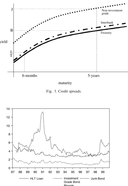
An explanation of the adjustment in square brackets in Eq. (3) is in order. The dependent variables in our tests are the changes in credit spreads (and, in the co-integrating relationship, the credit spreads themselves) over riskless funds for the appropriate duration. In calculating such a spread, one must be aware of two potential problems: (1) one should subtract oﬀ a true riskless cost of funds and (2) the instrument subtracted must be of the appropriate duration. Fig. 3 serves to illustrate the problems. HLT loans in our sample are priced at a spread over LIBOR. At any given rate setting date on a loan, LIBOR would be set as pointLin Fig. 3. But the true spread over riskless funds would be the quoted spread over six month LIBORplus

14We exclude those facilities not priced over Libor (e.g., facilities priced over prime, the CD rate, or those offering fixed interest rates or interest rate options). Initially, we classed the index into three sub- indices: investment-grade loan spread index, speculative-grade loan spread index and non-rated loan spread index according to the loan ratings assigned by S&P to the loans as reported by LPC. However as approximately 95% of the loans were un-rated and because the difference between spreads was small (averaging seven basis points between rated investment grade and rated sub-investment grade), we only report the total index results, not the result of sub-indices.

(14)

the spread of L–T. The L–Tspread represents the spread of unsecured short-term bank risk (typically Aa) over riskless funds. This spread has averaged 49 basis points over our sample period, but the margin ﬂuctuates (standard deviation of 0.28 basis

yield

maturity T

B J

L

6-months 5-years

Treasury Interbank

Non-investment grade

Fig. 3. Credit spreads.

0 2 4 6 8 10 12 14

87 88 89 90 91 92 93 94 95 96 97 98 99

HLT Loan Investment

Grade Bond Bbonds

Junk Bond

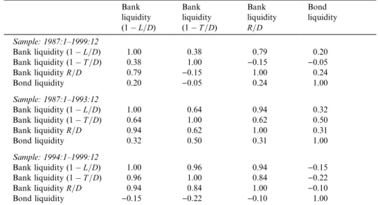
HLT Loan is the HLT loan spread as defined in equations 3 and 4

Investment Grade Bond is the yield to maturity on the index (the Lehman Brothers index) of Baa above investment grade bonds minus the yield to maturity of 5 year treasury bonds

Junk Bond is the yield to maturity on the index of non-investment grade bonds (the Lehman Brothers index) minus the yield to maturity of 5 year treasury bonds.

Fig. 4. Monthly spreads over treasury securities: HLT loan spread index, Lehman Brothers’ investment grade bond yield and Lehman Brothers’ high-yield bond yield.

(15)

Summary statistics

Period HLT

spread IG spread

Junk spread

Default TBill Yield curve

Loan liquidity (lL=D)

Loan liquidity (1T=D)

Bank liquidity (R=D)

Bond liquidity

1987:1–

1999:12

Mean 3.24 1.21 5.18 1.90 5.31 1.45 72.99 8.24 32.00 0.50

Median 3.02 1.22 4.79 1.50 5.10 1.30 72.52 9.62 31.90 0.95

Maximum 4.89 2.03 13.25 5.34 8.82 3.20 76.73 15.63 38.48 4.74

Minimum 2.52 0.72 2.58 0.54 2.61 )0.11 70.52 0.45 27.40 )8.14

Standard deviation

0.57 0.30 2.12 1.19 1.49 0.86 1.83 5.22 3.31 1.85

1987:1–

1993:12

Mean 3.49 1.37 6.29 2.52 5.72 1.72 73.08 12.51 30.44 0.21

Median 3.29 1.35 5.49 1.95 5.71 1.99 72.20 12.76 28.76 0.66

Maximum 4.89 1.87 13.25 5.34 8.82 3.20 76.73 15.63 37.52 4.74

Minimum 2.63 0.88 3.53 0.89 2.61 )0.11 70.52 9.06 27.40 )8.14

Standard deviation

0.65 0.21 2.27 1.27 1.91 0.87 2.20 2.16 3.30 2.15

1994:1–

1999:12

Mean 2.98 1.05 3.96 1.21 4.86 1.15 72.89 3.55 33.71 0.81

Median 2.91 0.96 3.65 1.06 4.98 1.03 72.55 2.54 32.78 1.10

Maximum 4.02 2.03 6.72 2.88 5.90 2.76 76.61 13.38 38.48 3.92

Minimum 2.52 0.72 2.58 0.54 3.03 )0.05 71.41 0.45 30.88 )3.83

Standard deviation

0.29 0.29 0.99 0.54 0.56 0.74 1.32 3.16 2.35 1.39

HTL spread¼the HLT loan spread as deﬁned by equations (3) and (4), IG spread¼the yield to maturity on the index of Baa investment grade bonds minus the yield to maturity of 5 year treasury bonds, junk spread¼the yield to maturity on the index of non-investment grade bonds minus the yield to maturity of 5 year treasury bonds, Default¼Moody’s monthly trailing 12-month default rates for all corporate, from http://riskcalc.moodysrms.com/us/research/def- rate.asp,tbill¼3 month t-bill return rate, yieldcurve¼5 years treasury bond yield maturity)3 months t-bill rate, bank liquidity (1L=D)¼1)(commercial and industrial loan)/deposits for all US commercial banks, bank liquidity (1T=D)¼1)(total loans and leases)/deposits for all US commercial banks, bank liquidity (R=D)¼(cash + US Government Securities)/deposits for all US commercial banks, bond liquidity¼net new purchases of bond mutual funds.

H.Thomas,Z.Wang/JournalofBanking&Finance28(2004)299–329313

(16)

points) and ranged from 16 to 145 basis points as spreads between Aa credits and treasuries ﬂuctuated.¹⁵ Concerning point (2), we calculate the long-term ﬁxed rate junk bond spread over a similar maturity treasury bond so that the spread over riskless funds is J–Busing the Datastream 5 year treasury yield.¹⁶

Fig. 4 plots the time trends of the three monthly spreads: HLT loans, junk bonds and investment grade bonds while Table 2 gives their summary statistics. Two facts are immediately apparent:

• The HLT loan spread is much less volatile and substantially lower than the junk bond spread and

• the HLT loan spread has roughly the same volatility but is substantially greater than the investment grade bond spread.

The HLT market’s lower volatility and correspondingly lower spread can be explained with the options pricing credit risk model that we refer to in the last section and that we theoretically prove in Appendix A. The HLT market’s relationship with the investment grade bond market spreads, however is not a matter of diﬀerential credit risk: senior HLT bank loan probabilities of default and losses given default are roughly comparable those of investment grade bonds (Altman and Suggitt, 2000). The higher spread is the price the borrower pays for ﬂexibility. Bank loans can be arranged quickly, involve closer relationships between bank and borrower and can generally be repaid without penalty prior to maturity.

6. Results

Table 3 shows the results of a contemporaneous regression of the change in the monthly HLT loan spread index calculated by us on the change in the Lehman Brothers junk bond and investment grade bond spreads. We conﬁrm Angbazo et al. (1998) results: the HLT loan spread is much more closely tied to the investment grade bond spread than to the junk bond spread. ¹⁷There is a substantial shift in the degree to which HLT loans spreads can be explained by investment grade bond spreads from the earlier seven years to the ﬁnal six years under study. As reference

15See Tuckman (1996) page 201. Another way to compare bond spreads with loan spreads would be to subtract the appropriate maturity interest rate swap rate from the fixed rate bond. Because the swap rate is swapped to LIBOR, it incorporates the AA risk spread in its pricing. This calculation would be similar to a company comparing two loan offers, a fixed rate offer and a floating rate offer on a swap- equivalent basis.

16To be accurate, one should use the spread of the zero coupon risky bond over the zero coupon treasury bond for each of the payments. Our use 5 year treasury bond yields is an approximation.

17The absolute magnitude of the co-movement of the investment grade bonds and HLT loan spread reported by Angbazo et al. (1998) was approximately 0.3, virtually identical to our 0.27 in panel 3 of Table 3, corresponding to the ﬁrst half of our sample (1987–1993) which coincides closely with the period in their study (1987–1994).

(17)

to the Chow test in the ﬁnal column in Table 3 shows, however, the change in re- gimes, while economically substantial, is not statistically signiﬁcant.

Although our contemporaneous first differences regression above suggests that there is a degree of bond and loan market integration and that the integration seems to be increasing, it tells us very little about the integration process. The first question is ‘‘are the spreads themselves co-integrated?’’ Fig. 4 suggests that the answer is ‘‘no’’

while Table 4 conﬁrms that suggestion. Using the Johansen test (Johansen, 1988, 1991), we are in general unable to reject the null hypothesis that no co-integration of the spreads occurs. In only one sub-period (1987–1993) for one pair (loan spreads and investment grade bond spreads) are we able to reject the hypothesis of no co-integration – with this rejection occurring at the 5% level. Statistical lack of co- integration of the spreads does not mean that the markets are not integrated. Partic- ularly, the spreads are determined in the diﬀerent market with respect to underlying

Table 3

Contemporaneous relationship between the HLT Loan, junk bond and investment bond spreads DHLT Spreadt¼a0þb1DJunk Spreadtþb2DIG Spreadtþet

Period DIG Spreadt DJunk Spreadt Constant R-squared CHOW test F-statistic (probability)

1987:1–1999:12 0.45 0.00 0.13

(4.27) (0.30)

1987:1–1993:12 0.40 )0.00 0.21 0.25

(3.47) ()0.35) (0.78)

1994:1–1999:12 0.51 0.01 0.10

(2.91) (0.53)

1987:1–1999:12 0.07 )0.00 0.03

(2.33) ()0.21)

1987:1–1993:12 0.06 )0.01 0.03 0.55

(1.60) ()0.69) (0.58)

1994:1–1999:12 0.10 0.01 0.04

(1.81) (0.53)

1987:1–1999:12 0.39 0.02 0.00 0.13

(2.71) (0.64) (0.34)

1987:1–1993:12 0.27 0.03 )0.00 0.24 0.33

(1.75) (1.19) ()0.19) (0.80)

1994:1–1999:12 0.55 )0.01 0.01 0.10

(2.22) ()0.23) (0.53)

DHLT Spreadtis the one month change in the HLT loan spread as deﬁned in Eqs. (3) and (4).DIG Spreadtis the one month change in the investment grade bond spread, being is the yield to maturity on the index of Baa investment grade bonds minus the yield to maturity of 5 year treasury bonds.DJunk Spreadtis the one month change in the junk bond spread, being the yield to maturity on the index of non-investment grade bonds minus the yield to maturity of 5 year treasury bonds. Chow test null hypothesis: no change in coeﬃcients from 1987–1993 to 1994–1999.

(18)

factors. When we include those underlying factors in the tests for co-integration, we ﬁnd co-integration in most data sets and their sub-periods, a result that leads us to the ECM. ¹⁸

Table 5 shows the results of our ECM model. The long-term effects are highly significant as evidenced by thet-statistic on the negative coefficient of the co-integrating vector, but the significance derives entirely from the latter period (with the coefficient on the vector on the first seven years being insignificant and taking the wrong sign).

Looking only at the 1994–1999 period, each month, spreads adjust about 24% of the diﬀerence from the long-term steady state spread. This suggests that 80% of the difference between the observed spread and modeled correct spread given default, liquidity and interest rate conditions would be dissipated within six months

Table 4

Co-integration test between HLT loan spreads and bond market yield spreads Variables Period Eigenvalue Likelihood

ratio

5% Critical value

1% Critical value

Hypothe- sized no. of CE(s) HLT spread

and IG spread

1987:1–1999:12 0.13 21.73 25.32 30.45 None

0.04 5.11 12.25 16.26 At most 1

1987:1–1993:12 0.35 29.39 25.32 30.45 None*

0.19 9.70 12.25 16.26 At most 1

1994:1–1999:12 0.13 16.83 25.32 30.45 None

0.09 6.42 12.25 16.26 At most 1

HLT spread and junk spread

1987:1–1999:12 0.05 14.18 25.32 30.45 None

0.04 5.75 12.25 16.26 At most 1

1987:1–1993:12 0.23 22.34 25.32 30.45 None

0.03 2.65 12.25 16.26 At most 1

1994:1–1999:12 0.15 16.47 25.32 30.45 None

0.07 4.96 12.25 16.26 At most 1

HLT spread and IG spread and junk spread

1987:1–1999:12 0.14 33.21 42.44 48.45 None

0.08 15.75 25.32 30.45 At most 1

1987:1–1993:12 0.25 39.40 42.44 48.45 None

0.16 16.84 25.32 30.45 At most 1

1994:1–1999:12 0.18 33.55 42.44 48.45 None

0.16 19.02 25.32 30.45 At most 1

HTL spread¼the HLT loan spread as deﬁned by Eqs. (3) and (4). IG spread¼the Lehman Brothers index of yield to maturity of Baa bonds minus the yield to maturity of the 5 year treasury bond. Junk Spread¼the Lehman Brothers index of yield to maturity of high-yield bonds minus the 5 year treasury bond. * denotes rejection of the hypothesis at 5% signiﬁcance level. None denotes the hypothesis of no co- integration relationship. At most 1 denotes the hypothesis of at most 1 co-integration relationship.

We omit tests of in excess of 1 co-integration relationship because failure to reject hypothesis of at most 1 co-integration relationship will also fail to reject higher levels of co-integration.

18We do not separately show test for co-integration of the spreads and the underlying factors. These tests are implicitly supplied by the signiﬁcance of the estimated coeﬃcient of the ECM in the following section.

(19)

(ð10:24Þ⁶¼0:19). Not surprisingly, as Panel B shows, the long-term eﬀect of high default rates is to increase spreads while the long-term eﬀect of high liquidity is to

Table 5

Error correction model: loan spread

DHLT Spreadt¼a0½HLT Spreadt1þb1defaultt1þb2tbillt1þb3yieldcurvet1þb4liquidityt1

þb5ðt1Þ þc þa1Ddefaultt1þa2Dtbillt1þa3Dyieldcurvet1þa4Dliquidityt1

þa5DHLT Spreadt1þConst Coeﬃcients 1987:1–

1999:12

1987:1–

1993:12

1994:1–

1999:12 PanelA: Coeﬃcients of one lag vector autoregression

a0 )0.10 0.01 )0.24

(0.03) (0.00) (0.08) ()3.27) (1.42) ()2.98) Ddefault_t1 )0.05 )0.03 )0.05

(0.10) (0.13) (0.18) ()0.47) ()0.21) ()0.30) Dtbill_t1 0.30 0.19 0.58

(0.08) (0.11) (0.16) (3.67) (1.72) (3.53) Dyieldcurvet1 )0.04 0.00 )0.04

(0.07) (0.12) (0.09) ()0.56) ()0.01) ()0.47) Dliquidityt1 )0.33 )0.59 )0.08

(0.11) (0.21) (0.13) ()3.01) ()2.79) ()0.60) DHLT Spreadt1 0.03 )0.03 0.20

(0.09) (0.12) (0.18) (0.32) ()0.23) (1.07)

Const 0.00 0.03 )0.01

(0.02) (0.03) (0.02) ()0.04) (0.95) ()0.39)

R² 0.16 0.14 0.26

PanelB: Components of the co-integrating vector

Spread default tbill yieldcurve liquidity trend C

1987:1–1999:12 1.00 )0.45 0.58 0.61 0.33 0.02 )32.13

(0.13) (0.16) (0.22) (0.06) (0.00)

1987:1–1993:12 1.00 5.48 )6.02 )5.83 )3.02 0.11 242.91

(16.55) (18.96) (17.43) (11.67) (0.48)

1994:1–1999:12 1.00 )0.14 0.12 0.42 0.00 0.00 )3.73

(0.10) (0.12) (0.14) (0.11) (0.01)

HTL Spread¼the HLT loan spread as deﬁned by equations (3) and (4), Default¼Moody’s monthly trailing 12-month default rates for all corporate, from http://riskcalc.moodysrms.com/us/research/def- rate.asp,tbill¼3 month t-bill return rate,yieldcurve¼5 years treasury bond yield maturity)3 months t-bill rate,liquidity¼1(commercial and industrial loan)/deposits for all US commercial banks. Standard errors are reported below each coeﬃcient.T-statistics are reported in panel A.

(20)

decrease spreads. Higher short-term interest rates and sharper yield curves are associated with long-term lower spreads, and in the long run, spreads are declining.¹⁹

Short-term dynamics are similarly logical. The short-term dynamics describe the effect of the previous month’s change in independent variables on the current month’s change on the loan spread.²⁰Here, only two effects are significant: short- term interest rates and liquidity. A rise in short-term interest rates leads to a substantial and significant rise in loanspreadsin the following month. In the latter period, a one percent rise in rates would be associated with a 58 basis point rise in spreads in the short run. A most interesting result concerns liquidity. Over the sample period, if bank liquidity rose by 10% (1 minus loans to deposit ratio increases by 0.1) spreads would fall in the next month by 0.03. But this effect is entirely explained by the first seven years. From 1994 to 1999, there is no significant effect of bank changes in liquidity on HLT loan spreads. ²¹

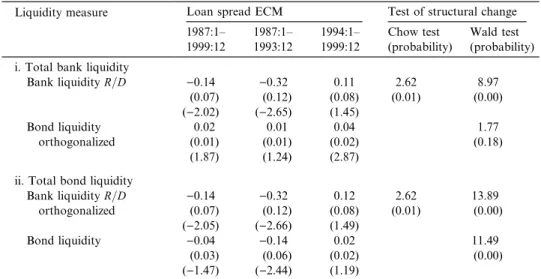
6.1. Interaction of liquidity in diﬀerent markets

Liquidity is at the heart of market integration. In the above analysis, we used the ECM to measure how liquidity (in addition to other factors) in the banking market affected the pricing of HLT loans. In this section, we consider how the liquidity of the junk bonds market, defined as net new purchases of junk bond mutual funds, ²²in addition to bank liquidity affects the pricing of HLT loans. In the above discussion we used only one definition of bank market liquidity: (1L=D) where L was the total commercial and industrial loans in the commercial banking system divided by total deposits. This adjusted ratio is also a measure of (unity minus) the portfolio proportionate allocation to a class of loans of which HLT loans is the most liquid component. To more closely approach a measure of gen- uine liquidity of commercial banks, we use two other measures, (1T=D) and R=D. In the former, T=D is the ratio of total loans and leases to deposits, while the latter is a measure of reserves to deposits, being cash plus US government securities over deposits.

19The reader will note that, although in Table 5 Panel B, we display standard errors for the coefficients of variables in the co-integrating vector, we do not displayt-statistics. Those variables’ distributions do not follow a simple distribution so their critical values are not known. Although one can make statements about the significance of the whole co-integrating vector, one cannot about the significance of its individual components. See Johansen (1991).

20Clearly, our model captures only the one-month lag cause and eﬀect. To the extent that loan market pricing reactions between changes in underlying economic factors occur in a shorter time horizon, our one month ECM is unable to explain the changes in spreads. This may help explain the lowR².

21Although this change in coefficient itself is significant, using a Chow test (F ¼0:84) one is unable to reject the null hypothesis that there has been a change in theentiremodel coefficients from the first sub- period to the second.

22This is clearly not the only variable that could be used to deﬁne junk bond market liquidity. We ran the regressions with a second variable, the percentage of cash in junk bond mutual fund portfolios. The orthoganalized results were not substantially diﬀerent to those described in this section.