WHAT DO WE KNOW AND WHAT ARE THE IMPLICATIONS?

(1)

WHAT DO WE KNOW AND WHAT ARE THE IMPLICATIONS?

Susan Sunila Sharma¹, Lutzardo Tobing², Prayudhi Azwar³

1 Department of Finance & Centre for Financial Econometrics, Deakin Business School, Australia.

Email: s.sharma@deakin.edu.au

2 Bank Indonesia Institute, Bank Indonesia, Jakarta, Indonesia. Email: lutzardo@bi.go.id

3 Bank Indonesia Institute, Bank Indonesia, Jakarta, Indonesia. Email: yudhi@bi.go.id

Unit root properties of macroeconomic data are important for both econometric modeling and policymaking. The form of variables (whether they are a unit root process) helps determine the correct econometric model. Equally, the form of variables helps explain how they react to shocks (both internal and external). Macroeconomic time-series data are often at the forefront of shock analysis and econometric modeling.

There is a growing research emphasis on Indonesia using time-series data; yet, there is limited understanding of the data characteristics and shock response of these data.

Using an extensive dataset comprising 33 macroeconomic time-series variables, we provide an informative empirical analysis of unit root properties of this data. We find that, regardless of data frequency, empirical evidence of unit roots is mixed.

Some data series respond quickly to shocks while others take more time. Almost all macroeconomic data suffer from structural breaks. We draw implications from these findings.

Keywords: Unit root; Macroeconomic data; Structural breaks; Shocks; Econometric modeling.

JEL Classification: C5; E1.

ABSTRACT

Article history:

Received : July 1, 2018 Revised : October 20, 2018 Accepted : October 20, 2018 Available online : October 31, 2018 https://doi.org/10.21098/bemp.v21i2.967

(2)

policymakers interpret and use data. URP assists in understanding the form of data. There are two forms data can take, either stationary or non-stationary.

In simple terms, stationary time-series data have mean, variance, and co-variance that do not change over time. By comparison, a non-stationary series is best characterized as one whose mean, variance, and co-variance change over time.

Precise knowledge of the form of the time-series data is important, because when its form is stationary, this implies that shocks will have short-term (or temporary) effects. On the other hand, a non-stationary series implies that shocks have long-term or permanent effects on the variable. This knowledge has policy implications because policymakers need to understand the form of variables to deduce how they will react to policy changes and/or shocks.

The second advantage from understanding the form of variables has roots in econometric modeling. Applied researchers are constrained by theory in modeling data. Theory also tends to dictate the form in which variables need to be modeled.

There are many examples of this. Two are offered here for demonstration. First, consider the Purchasing Power Parity (PPP) hypothesis, which holds that prices equalize across countries, meaning that any price differences on a good/service in any two like countries should be stationary for PPP to hold; see Narayan (2006a).

Second, the popular efficient market hypothesis argues that asset prices (such as stock prices) should be stationary (see Narayan and Smyth, 2007).

So great has been the influence of unit roots pioneered by Nelson and Plosser (1982)—considering the need to understand the shock reaction of variables and the form in which they enter econometric modeling, as discussed above—that there is a separate literature on new tests for unit roots; see also Perron (1989), which marks the starting point for research based on structural break(s). In other words, researchers have focused attention on developing more robust unit root tests that can offer greater precision when testing for the precise form of the data. Two avenues for improvement noted recently are important to highlight.

Endogenous structural break treatment has a notable history in unit root testing.

However, while the tests became available following Lee and Strazicich (2003), subsequent work (see, for instance, Narayan and Popp, 2010) took issue with the precision in estimating the break dates themselves, because accurate identification of breaks has implications for precise understanding of the form of the data (Narayan and Popp, 2010). More recent work (Narayan and Liu, 2015; Narayan, Liu and Westerlund, 2016) takes issue with the fact that when modeling for unit roots, it is not only structural breaks that are important, but also the role of a time trend and data heteroskedasticity can be equally important in delivering an unbiased understanding of the data.

Macroeconomic data are also important for Indonesia. Several studies analyze Indonesian macroeconomic data via testing different relations. For instance, Amir, Asafu-Adjaye, and Ducpham (2013) examine the impact of Indonesia’s income tax reforms on various macroeconomic variables, namely real Gross Domestic Product (GDP), real private consumption, real investment, real government consumption, real exports, real imports, consumer price index,

(3)

on the market and firm-level liquidity of eight emerging stock markets in Asia.

Tanuwidjaja and Choy (2006) examine the role of Indonesian central bank credibility in achieving an inflation target. Hadiwibowo and Komatsu (2011) examine the macroeconomic trilemma and international capital flows under several financial structures in Indonesia. Djuranovik (2014) develops a model of the term structure of interest rates in Indonesia to create a link between the yield curve and macroeconomic fundamentals, namely real activity, inflation, and interest rate. Sowmya and Prasanna (2018) examine interaction between the yield curve and macroeconomic factors of Asian economies. Such studies and future research would benefit from greater understanding of the importance of unit root tests.

Returning to the idea of understanding the form of the variable, what started off as instrumental knowledge in using macroeconomic data spread quickly to other fields of research where shocks were relevant in understanding how variables respond to them. The unit root idea, for instance, was popularized in Narayan and Smyth (2007) in a time-series setting and extended to a panel data setting in Narayan, Narayan, and Smyth (2008). In tourism economics, the idea was introduced by Narayan (2005a,b) and in health economics by Narayan (2006b). The main message of these studies is that unit root evidence is important to understanding the nature and impact of shocks not only with macroeconomic data (see Section II), but also with other time-series data where shocks are relevant, such as in energy, tourism, and health.

This paper proceeds as follows. Section II reviews the literature on the presence of unit root in macroeconomic data. Section III discusses our data and results.

Finally, Section IV sets forth concluding remarks.

II. THE LITERATURE

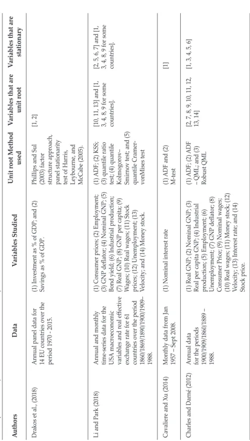
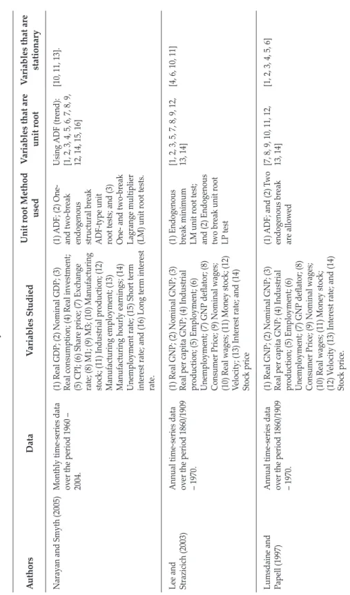
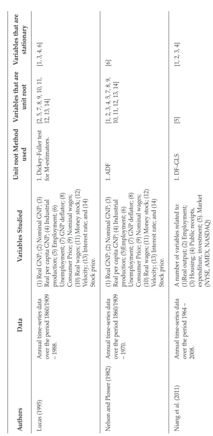
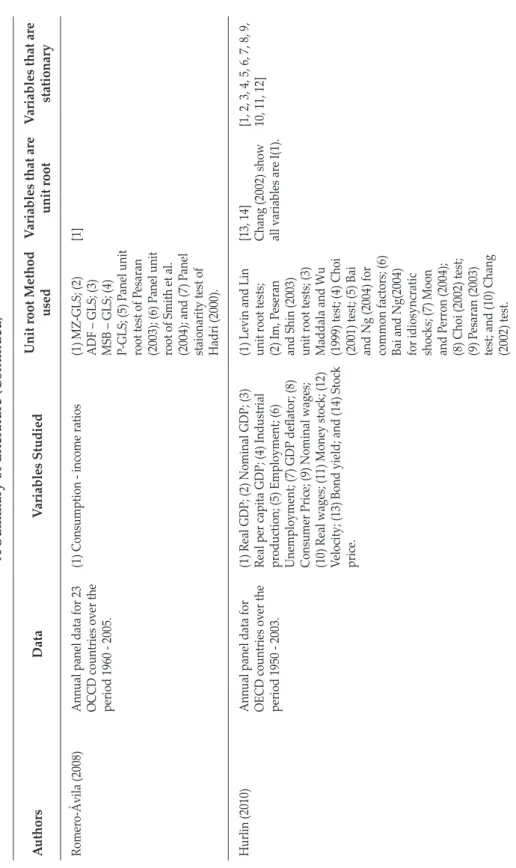
This section provides a feel for the importance of understanding the unit root behavior of macroeconomic data. We choose selected studies from this literature that we believe best offers a snapshot of the work done on unit roots devoted to macroeconomic data.

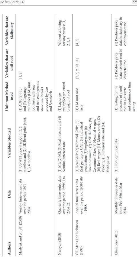
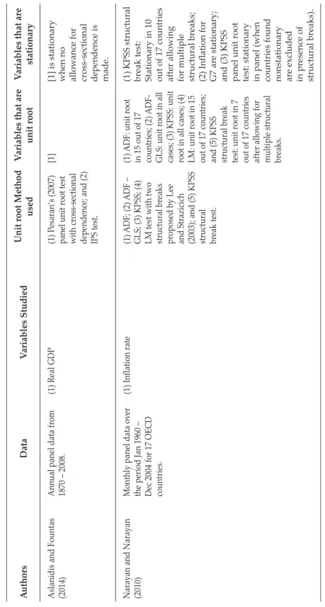
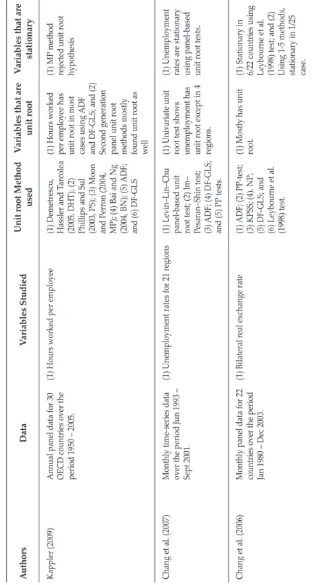
Table 1 summarizes selected literature on unit roots. We believe that these studies provide a reasonable representation of the literature and the features that characterize this literature. Let us identify these features more precisely. First, note from Column 2 that unit root tests of macroeconomic data are conducted at different data frequencies (annually, weekly, quarterly, and monthly), although most work seems to use annual data followed by monthly data. The dominance of annual data is expected given that, for most countries, macroeconomic data (over time) is available only annually. One issue arising from this concerns robustness. The question arises of whether the evidence on unit root data is frequency-dependent.

We address this by undertaking a unit root test on both annual and monthly data. A caveat here is that one ends up with different start dates when using

(4)

we have some results that we can consider, depending on policy objectives.

The second feature of the literature, which can be read from Column 3, is that a wide range of macroeconomic data are utilized in unit root tests. The most popular data series seem to be GDP, inflation, and exchange rate; the highest number of variables used is around 14. Our study presents an extensive unit root analysis focusing on Indonesia—our sample includes 33 annual time-series data and 31 monthly time-series data. This represents a first comprehensive analysis of unit root testing of macroeconomic data.

The third feature concerns the econometric approach taken to test the unit root hypothesis. There are several points to note here. First, early studies seem to use tests without structural breaks. These studies are complemented by papers that address the unit root issue with structural breaks. Second, recent studies employ panel data models. Thus, the literature has progressed from time-series–

based methods to panel data–based methods for testing the unit root hypothesis.

We position our study within the popular structural break unit root testing methodology.

The final feature concerns the evidence on unit root. At best, the evidence appears mixed. Two trends are notable, however. First, panel data models offer greater evidence of stationarity. One reason for this is the gain in power to reject the unit root null that results from an increase in sample size when data is pooled across cross-sections and over time. Second, time-series models that accommodate structural break(s) offer greater evidence of stationarity (evidence against the unit root null hypothesis). These factors have implications for how one should approach unit root testing in macroeconomic data. We employ structural break unit roots tests within a time-series setting.

III. DATA AND RESULTS

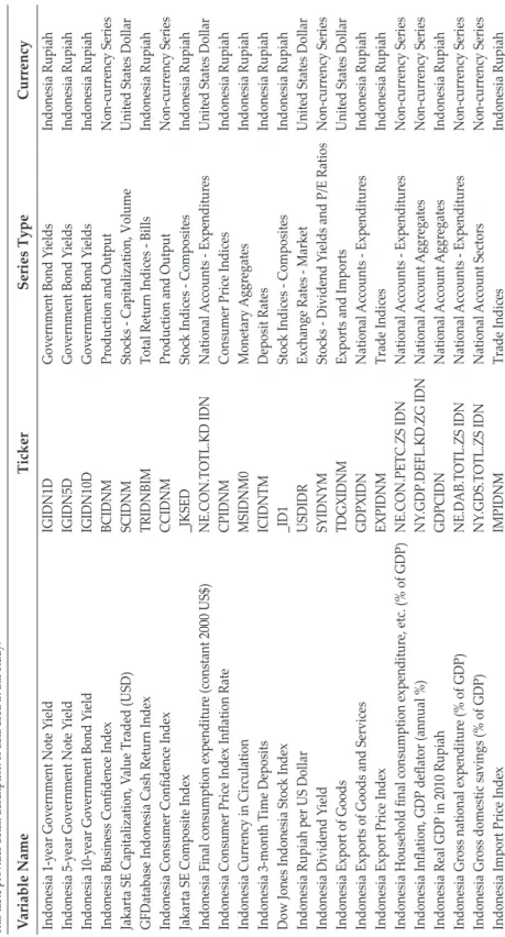
Time-series data are used for unit root testing. A total of 31 monthly and 33 annual time-series macroeconomic variables for Indonesia are employed in this study. A complete list of variables is provided in Tables 2 (monthly series) and 3 (annual series). In summary, our dataset has three bond yield variables (separated by maturity), four interbank interest rate variables (separated by maturity), nine financial variables (business confidence index, capital value added, cash return index, dividend yield, Dow Jones stock index, market capitalization to GDP, Jakarta stock exchange Islamic index, price-to-earnings ratio, stock return index), and 17 monetary/trade-related variables (CPI, deposit rate, industrial production, composite index, exchange rate, export goods, export index, import goods, import index, industrial production, lending rate, M1, M2, producer price index, foreign exchange reserves, unemployment, and wholesale price index). All data are obtained from the Global Financial Database.

(5)

This table provides summary of literature on studies that examine the presence of unit root in macroeconomic variables. AuthorsDataVariables StudiedUnit root Method usedVariables that are unit rootVariables that are stationary Drakos et al., (2018) Annual panel data for 14 EU countries ov

er the period 1970 - 2015.

(1) Investment as % of GDP; and (2) Savings as % of GDP.

Phillips and Sul (2003) factor structure approach, panel stationarity test of Harris, Leybourne, and McCabe (2005).

[1, 2] Li and Park (2018)

Annual and monthly time-series data for the USA macroeconomic variables and real effectiv

e

exchange rate for 61 countries ov

er the period

1860/1869/1890/1900/1909– 1988.

(1) Consumer prices; (2) Employment; (3) GNP deflator; (4) Nominal GNP; (5) Bond yield; (6) Industrial production; (7) Real GNP; (8) GNP per capita; (9) Wages; (10) Real wages; (11) Stock prices; (12) Unemployment; (13) Velocity; and (14) Money stock.

(1) ADF; (2) KSS;

(3) quantile ratio test; (4) quantile Kolmogorov– Smirnov test; and (5) quantile Cramer- vonMises test [10, 11, 13] and [1, 3, 4, 8, 9 for some countries].

[2, 5, 6, 7] and [1, 3, 4, 8, 9 for some countries].

Cavaliere and Xu (2014)

Monthly data from Jan 1957 – Sept 2008.

(1) Nominal interest rate(1) ADF and (2) M-test[1] Charles and Darné (2012)

Annual data for the periods 1900/1909/1860/1889 – 1988.

(1) Real GNP; (2) Nominal GNP; (3) Real per capita GNP; (4) Industrial production; (5) Employment; (6) Unemployment; (7) GNP deflator; (8) Consumer Price; (9) Nominal w ages; (10) Real wages; (11) Money stock; (12)

Velocity; (13) Interest rate; and (14) Stock price.

(1) ADF; (2) ADF

– QML; and (3) Robust QML [2, 7, 8, 9, 10, 11, 12, 13, 14]

[1, 3, 4, 5, 6]

Table 1. A Summary of Literature

(6)

AuthorsDataVariables StudiedUnit root Method usedVariables that are unit rootVariables that are stationary Narayan and Smyth (2005)

Monthly time-series data over the period 1960 – 2004.

(1) Real GDP; (2) Nominal GDP; (3) Real consumption; (4) Real inv

estment;

(5) CPI; (6) Share price; (7) Exchange rate; (8) M1; (9) M3; (10) Manufacturing stock; (11) Industrial production; (12) Manufacturing employment; (13) Manufacturing hourly earnings; (14) Unemployment rate; (15) Short term interest rate; and (16) Long term interest rate.

(1) ADF; (2) One-

and two-break endogenous structural break ADF-type unit root tests; and (3) One- and two-break Lagrange multiplier (LM) unit root tests.

Using ADF (trend):

[1, 2, 3, 4, 5, 6, 7, 8, 9, 12, 14, 15, 16]

[10, 11, 13].

Lee and Strazicich (2003)

Annual time-series data over the period 1860/1909 – 1970.

Velocity; (13) Interest rate; and (14) Stock price

(1) Endogenous break minimum LM unit root test; and (2) Endogenous two break unit root LP test

[1, 2, 3, 5, 7, 8, 9, 12, 13, 14]

[4, 6, 10, 11]

Lumsdaine and Papell (1997)

(1) Real GNP; (2) Nominal GNP; (3) Real per capita GNP; (4) Industrial production; (5) Employment; (6) Unemployment; (7) GNP deflator; (8) Consumer Price; (9) Nominal w

ages; (10) Real wages; (11) Money stock; (12) Velocity (13) Interest rate; and (14) Stock price.

(1) ADF; and (2) Two

endogenous break are allow

ed

[7, 8, 9, 10, 11, 12, 13, 14]

[1, 2, 3, 4, 5, 6]

Table 1. A Summary of Literature (Continued)

(7)

Table 1. A Summary of Literature (Continued) AuthorsDataVariables StudiedUnit root Method usedVariables that are unit rootVariables that are stationary Lucas (1995)

1. Dickey-Fuller test for M-estimators.

[2, 5, 7, 8, 9, 10, 11, 12, 13, 14]

[1, 3, 4, 6] Nelson and Plosser (1982)

(1) Real GNP; (2) Nominal GNP; (3) Real per capita GNP; (4) Industrial production; (5)Employment; (6) Unemployment; (7) GNP deflator; (8) Consumer Price; (9) Nominal w ages; (10) Real wages; (11) Money stock; (12)

1. ADF

[1, 2, 3, 4, 5, 7, 8, 9, 10, 11, 12, 13, 14]

[6] Niang et al. (2011)

Annual time-series data over the period 1964 – 2008.

A number of variables related to:

(1)Real output; (2) Employment; (3) Housing; (4) Public receipts, expenditure, inv estment; (5). Market (NYSE, AMEX, NASDAQ)

1. DF–GLS[5][1, 2, 3, 4]

(8)

AuthorsDataVariables StudiedUnit root Method usedVariables that are unit rootVariables that are stationary Romero-Ávila (2008) Annual panel data for 23 OCCD countries ov

(1) Consumption - income ratios

(1) MZ-GLS; (2) ADF – GLS; (3) MSB – GLS; (4) P-GLS; (5) P

anel unit root test of Pesaran (2003); (6) Panel unit

root of Smith et al. (2004); and (7) P

anel

staionarity test of Hadri (2000).

[1] Hurlin (2010)

Annual panel data for OECD countries ov

(1) Real GDP; (2) Nominal GDP; (3) Real per capita GDP; (4) Industrial production; (5) Employment; (6) Unemployment; (7) GDP deflator; (8) Consumer Price; (9) Nominal w ages; (10) Real wages; (11) Money stock; (12)

Velocity; (13) Bond yield; and (14) Stock price.

(1) Levin and Lin unit root tests; (2) Im, P

eseran

and Shin (2003) unit root tests; (3) Maddala and Wu (1999) test; (4) Choi (2001) test; (5) Bai and Ng (2004) for common factors; (6) Bai and Ng(2004) for idiosyncratic shocks; (7) Moon and P

erron (2004);

(8) Choi (2002) test; (9) P

esaran (2003)

test; and (10) Chang (2002) test.

[13, 14] Chang (2002) show all v

ariables are I(1).

[1, 2, 3, 4, 5, 6, 7, 8, 9, 10, 11, 12]

(9)

AuthorsDataVariables StudiedUnit root Method usedVariables that are unit rootVariables that are stationary Maslyuk and Smyth (2008)Weekly time-series data over the period 1991 – 2004.

(1) US WTI price at (spot, 1, 3, 6 months); and (2) UK Brent price (spot, 1, 3, 6 months).

(1) ADF; (2) PP;

and (3) Lagrange multiplier (LM) unit root tests with one and

two endogenous

structural breaks proposed by Lee and Strazicich

[1, 2] Narayan (2008)

Quarterly time-series data over the period 1959:01 to 2004:02.

(1) M1; (2) M2; (3) Real income; and (4) Nominal interest rate (1) Lagrange multiplier structural break unit root

Without allowing

for any breaks: [1, 2, 3, 4]

Gil-Alana and Robinson (1997)

(1) Real GNP; (2) Nominal GNP; (3) Real per capita GNP; (4) Industrial production; (5)Employment; (6) Unemployment; (7) GNP deflator; (8) Consumer Price; (9) Nominal w ages; (10) Real wages; (11) Money stock; (12)

(1) LM unit root tests[7, 8, 9, 10, 11][4, 6] Chambers (2015)

Monthly time-series data from Feb 1996 to Mar 2014.

(1) Producer price data(1) Testing for the

presence of a unit root in a discrete and continuous time setting (1) Producer price data has unit root in discrete time.

(1) Producer price data is stationary in continuous time.

(10)

AuthorsDataVariables StudiedUnit root Method usedVariables that are unit rootVariables that are stationary Aslanidis and Fountas (2014) Annual panel data from 1870 – 2008.

(1) Real GDP(1) Pesaran’s (2007)

panel unit root test with cross-sectional dependence; and (2) IPS test.

[1]

[1] is stationary when no allow

ance for

cross-sectional dependence is made.

Narayan and Narayan (2010)Monthly panel data over the period Jan 1960 – Dec 2004 for 17 OECD countries.

(1) Inflation rate(1) ADF; (2) ADF –

GLS; (3) KPSS; (4) LM test with two structural breaks proposed by Lee and Strazicich (2003); and (5) KPSS structural break test.

(1) ADF: unit root

in 15 out of 17 countries; (2)

ADF-

GLS: unit root in all cases; (3) KPSS: unit root in all cases; (4) LM: unit root in 15 out of 17 countries; and (5) KPSS structural break test: unit root in 7 out of 17 countries after allowing for multiple structural breaks.

(1) KPSS structural

break test: Stationary in 10 out of 17 countries after allowing for multiple structural breaks; (2) Inflation for G7 are stationary; and (3) KPSS panel unit root test: stationary in panel (when countries found nonstationary are excluded in presence of structural breaks).

(11)

AuthorsDataVariables StudiedUnit root Method usedVariables that are unit rootVariables that are stationary Kappler (2009) Annual panel data for 30 OECD countries ov

er the period 1950 – 2005.

(1) Hours worked per employee

(1) Demetrescu, Hassler and T

arcolea

(2005, DHT); (2) Phillips and Sul (2003, PS); (3) Moon and P

erron (2004,

MP); (4) Bai and Ng (2004, BN); (5)

ADF; and (6) DF-GLS

(1) Hours worked per employ

ee has

unit root in most cases using

ADF

and DF-GLS; and (2) Second generation panel unit root methods mostly found unit root as well

(1) MP method rejected unit root hypothesis

Chang et al. (2007)

Monthly time-series data over the period Jun 1993 – Sept 2001.

(1) Unemployment rates for 21 regions

(1) Levin–Lin–Chu panel-based unit root test; (2) Im– Pesaran–Shin test; (3) ADF; (4) DF-GLS; and (5) PP tests.

(1) Univariate unit

root test shows unemployment has unit root except in 4 regions.

(1) Unemployment rates are stationary using panel-based unit root tests.

Chang et al. (2006)

Monthly panel data for 22 countries ov

er the period Jan 1980 – Dec 2003.

(1) Bilateral real exchange rate(1) ADF; (2) PP-test;

(3) KPSS; (4). NP; (5) DF-GLS; and (6) Leybourne et al. (1998) test.

(1) Mostly has unit root.

(1) Stationary in 6/22 countries using Leybourne et al. (1998) test; and (2) Using 1-5 methods, stationary in 1/25 case.

(12)

AuthorsDataVariables StudiedUnit root Method usedVariables that are unit rootVariables that are stationary Hüseyin (2005) Monthly time-series data for the USA, UK, Germany, and Italy ov

er

the period Jan 1982 – Dec 2003.

(1) Bilateral real exchange rate(1) ADF; (2) PP-

test; (3) KPSS; (4) Modified Ng and Perron test.

(1) Maximum presence of unit root in the case of Germany and Italy.

(1) Maximum cases of stationarity for the USA and UK.

Smyth (2003)

Quarterly panel data for 6 Australian state and 2 territories over the period Feb 1982 – Jan 2002.

(1) Unemployment rates(1) ADF; (2) Levin- Lin and FGLS Tests; and (3) IPS Test.

Both ADF and IPS

finds [1] to be a stationary v

ariable.

Levin and Lin (1992) and FGLS test show presence of unit root in [1].

Choi (2001)Monthly panel data over

the period Mar 1973 – Mar 1996.

(1) Real exchange rates (US real exchange rates vs. the Canadian dollar; German Mark; Japanese Y

en; French

Franc; British Pound; and the Swiss Franc).

(1) DF-GLS; and (2) combination unit root tests and IPS’ t-bar test.

(1) DF-GLS shows unit root in Exchange rates (1) Combination unit root tests and IPS’ t-bar test shows some evidence of stationarity.

(13)

null hypothesis of a normal distribution.

No. Series Sample Period Obs. Mean Std. Dev. Skewness Jarque-Bera p-value 1 Bond Yield, 3 Year 2009:05-2018:06 110 1.814 0.178 -0.672 9.194 0.010 2 Bond Yield, 5 Year 2009:05-2018:06 110 1.952 0.182 -0.453 5.342 0.069 3 Bond Yield, 10 Year 2009:05-2018:06 110 2.019 0.170 -0.125 0.794 0.672 4 Business Confidence

Index 2002:01-2017:12 190 4.602 0.010 -1.526 97.560 0.000

5 Capital Value Traded 1990:01-2018:05 341 11.288 1.334 -0.235 16.770 0.000 6 Cash Return Index 1989:12-2018:06 343 4.480 1.122 -0.513 34.768 0.000 7 Composite Index 1983:03-2018:06 424 6.582 1.365 -0.073 16.025 0.000 8 Consumer Confidence

Index 2001:04-2017:12 201 4.601 0.013 -1.062 56.344 0.000

9 CPI Inflation 1967:01-2018:06 618 2.630 1.615 -0.333 32.348 0.000 10 Deposit Rate 1974:04-2016:07. 508 2.421 0.495 0.364 16.186 0.000 11 Dividend Yield 1990:11-2018:06 332 0.598 0.651 -2.934 1850.536 0.000 12 Exchange Rate 1876:01-2018:06 1710 -0.629 6.495 0.519 259.035 0.000 13 Dow Jones Stock Index 1992:01-2018:06 318 5.982 0.836 0.152 33.685 0.000 14 Export Goods 1961:01-2018:05 689 9.772 1.846 -0.617 65.459 0.000 15 Export Index 1991:01-2018:05 329 -0.304 0.289 0.040 20.510 0.000 16 GFD Market

Capitalisation of GDP 1995:01-2018:05 281 -7.049 1.534 0.672 58.232 0.000 17 Import Goods 1960:01-2018:06 701 9.426 1.856 -0.370 46.696 0.000 18 Import Index 1991:01-2018:05 329 -0.295 0.324 -0.641 25.998 0.000 19 Indonesia 1 Month

Interbank Interest Rate (JIBOR)

1990:01-2018:06 342 2.357 0.546 0.914 73.150 0.000

20 Indonesia 3 Month Interbank Interest Rate (JIBOR)

1993:12-2018:06 295 2.340 0.526 0.996 64.297 0.000

21 Indonesia 6 Month Intebank Interest Rate (JIBOR)

1991:01-2018:06 330 2.382 0.478 0.779 39.274 0.000

22 Indonesia 12 Month Intebank Interest Rate (JIBOR)

1997:03-2018:06 256 2.334 0.484 1.127 66.305 0.000

23 Industrial Production

Volume 1991:12-2018:04 317 12.579 0.224 0.208 8.340 0.015

24 Jakarta Stock Exchange

Islamic Index 2000:07-2018:06 216 5.700 0.861 -0.715 26.511 0.000 25 Lending Rate for

Working Capital 1986:03-2016:08 366 2.860 0.275 0.316 10.954 0.004 26 M1-Money Supply 2008:01-2018:04 124 13.550 0.366 -0.150 8.081 0.018 27 M2-Money supply 200:801-2018:04 124 14.965 0.374 -0.234 9.233 0.010

(14)

Table 3.

Descriptive Statistics of Yearly Data

No. Series Sample Period Obs. Mean Std. Dev. Skewness Jarque-Bera p-value 28 Price to Earnings Ratio 1990:01-2018:06 342 2.813 0.342 0.049 32.162 0.000 29 Producer Price Index

Excluding Oil 1971:01-2016:04 544 2.604 1.575 -0.200 26.700 0.000 30 Stock Return Index 1988:01-2018:06 366 7.637 1.286 0.153 22.583 0.000 31 Total Foreign

Exchange Reserves (exclude Gold)

1971:01-2018:06 570 9.383 1.659 -0.478 24.609 0.000

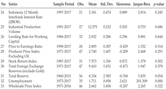
This table presents descriptive statistics for yearly data. Thirty-three data series are considered, and Column 3 contains the sample period for each series followed by the number of observations (Obs.) in the sample. The mean, Standard Deviation (SD), skewness, Jarque–Bera (JB) test coefficient and its respective p-values are presented in Columns 5 to 9, respectively. The JB test examines the null hypothesis of a normal distribution.

No Series Sample Period Obs. Mean Std. Dev. Skewness Jarque-Bera p-value 1 Capital Value Traded 1977-2017 41 9.119 3.556 -0.665 4.758 0.093

2 Cash Return Index 1989-2017 29 4.443 1.164 -0.494 2.929 0.231

3 Composite Index 1977-2017 41 6.305 1.448 0.174 2.463 0.292

4 CPI 1960-2016 57 1.626 3.295 -1.647 36.827 0.000

5 CPI Inflation 1948-2017 70 -0.351 5.297 -0.955 12.002 0.002

6 Deposit Rate 1974-2017 44 2.406 0.502 0.514 1.974 0.373

7 Dividend Yield 1990-2017 28 0.585 0.696 -2.858 132.257 0.000

8 Dow Jones Stock Index 1992-2017 26 5.991 0.849 0.113 2.676 0.262

9 Exchange Rate 1818-2017 200 -2.170 6.002 1.058 41.992 0.000

10 Export Goods 1946-2017 72 9.102 2.191 -0.251 5.507 0.064

11 Export Goods and Services 1990-2017 28 13.221 1.256 -0.393 2.339 0.311

12 Export Index 1991-2017 27 -0.299 0.284 0.071 1.951 0.377

13 GDP-Deflator Inflation 1961-2015 55 2.758 1.100 0.970 8.970 0.011

14 GDP-Deflator 1960-2015 56 1.671 2.166 -0.278 2.359 0.307

15 GFD Market Capitalisation

of GDP 1993-2017 25 -6.875 1.591 0.612 4.731 0.094

16 Nominal GDP 1951-2017 67 9.383 6.128 -0.850 9.208 0.010

17 Real GDP 1870-2017 148 13.421 1.263 0.634 14.674 0.001

18 Import Goods 1946-2017 72 8.847 2.111 -0.048 5.574 0.062

19 Import Goods and Services 1990-2017 28 13.221 1.256 -0.393 2.339 0.311

20 Import Index 1991-2017 27 -0.280 0.307 -0.458 2.140 0.343

1990-2017 28 2.366 0.503 0.523 1.281 0.527

1993-2017 25 2.361 0.506 0.708 2.202 0.332

1991-2017 27 2.383 0.471 0.728 2.732 0.255

(15)

A plot of the annual time-series data is available in Figure 1. Tables 2 and 3 show descriptive statistics based on monthly and annual time-series data, respectively. Given the time-series nature of the data, we note from both these tables the start data. Not all series have lengthy data. For example, some series, like exchange rate, have data going as far back as 1876. Inflation and deposit rate data are available from the 1960s and 1970s, respectively, while for other series much smaller data samples are available. Details are found in Columns 2 and 3 of these tables. Thus, data series have different start dates. This is dictated entirely by data availability.

1997-2017 21 2.341 0.474 0.889 2.814 0.245

Volume 1991-2017 27 12.575 0.232 0.203 0.753 0.686

26 Lending Rate for Working

Capital 1986-2017 32 2.832 0.286 0.296 0.881 0.644

27 Price to Earnings Ratio 1990-2017 28 2.805 0.307 -0.429 1.332 0.514 28 Producer Price Index

Excluding Oil 1971-2017 47 2.740 1.607 -0.209 2.468 0.291

29 Stock Return Index 1987-2017 31 7.573 1.356 0.072 1.378 0.502 30 Total Foreign Exchange

Reserves (exclude Gold) 1971-2017 47 9.410 1.651 -0.473 1.947 0.378

31 Total Reserve 1960-2015 56 8.334 2.585 -0.768 5.835 0.054

32 Unemployment 1973-2017 35 1.711 0.858 2.621 201.509 0.000

33 Wholesale Price Index 1971-2016 46 2.662 1.604 -0.207 2.265 0.322

Figure 1. A Plot of Annual Time-Series Data Cash Return Index

0 10

1989 1994 1999 2004 2009 2014

This figure plots annual time-series data for 33 variables. Full variable description is given in Appendix Table A1. The time-span of each variable is dependent on data availability and is explicitly noted in Tables 2-3.

(16)

Composite Index

0 5 10

1977 1983 1989 1995 2001 2007 2013

Capital Value

0 10 20

1977 1983 1985 1995 2004 2013

CPI Inﬂation

-20 -10 0 10

1948 1962 1976 1990 2004

(17)

-10 0 10

1818 1852 1886 1920 1954 1988

Deposit Rate

0 2 4 6

1974 1981 1988 1995 2002 2009 2016

Dow Jones Indonesia

0 5 10

1992 1998 2004 2010 2016

(18)

Dividend Yield

-4 -2 0 2

1990 1996 2002 2008 2014

6-month JIBOR

0 2 4

1991 1996 2001 2006 2011 2016

Market Capitalization

-10 -5 0

1993 1998 2003 2008 2013

(19)

11 12 13

1991 1997 2003 2009 2015

0 2 4

1990 1994 1998 2002 2006 2010 2014

1-month JIBOR

3-month JIBOR

0 2 4

1993 1998 2003 2008 2013

(20)

Price to Earning Ratio

0 2 4

1990 1994 1998 2002 2006 2010 2014

0 2 4

1986 1991 1996 2001 2006 2011 2016

Lending Rate

12-month JIBOR

0 2 4

1997 2000 2003 2006 2009 2012 2015

(21)

0

1971 1979 1987 1995 2003 2011

0 20

1870 1895 1920 1945 1970 1995

Real GDP

Wholesale Price Index

-5 0 5 10

1971 1979 1987 1995 2003 2011

(22)

0 20

1987 1993 1999 2005 2011 2017

Stock Index

Producer Price Index

-5 0 5 10

1971 1979 1987 1995 2003 2011

0 10 20

1946 1958 1970 1982 1994 2006

Export Goods

(23)

0 10

1990 1995 2000 2005 2010 2015

-1 0 1

1991 1996 2001 2006 2011 2016

Export Index

0 5 10

1983 1989 1995 2001 2007 2013

Unemployment

(24)

0 10 20

1946 1958 1970 1982 1994 2006

Import Goods

-1 0 1

1991 1996 2001 2006 2011 2016

Import Index

0 20

1990 1995 2000 2005 2010 2015

Import Goods & Services

(25)

-10 -5 0 5

1960 1972 1984 1996 2008

-10 0 10 20

1951 1965 1979 1993 2007

Nominal GDP

-5 0 5

10 GDP-Deﬂator

1960 1965 1970 1975 1980 1985 1990 1995 2000 2005 2010 2015

(26)

0 5 10

1961 1966 1971 1976 1981 1986 1991 1996 2001 2006 2011

GDP Deﬂator Inﬂation

0 10 20

1960 1966 1972 1978 1984 1990 1996 2002 2008 2014

Total Reserve

The Narayan and Popp (2010) test results for monthly data are reported in Table 4. We document that regardless of the type of model specification (i.e., Model 1 or Model 2), the unit root null hypothesis with monthly data is rejected for business confidence index, capital value traded, cash return index, consumer confidence index, exchange rate, 1- and 3-month interbank interest rate, industrial production (volume), lending rate, M1, price-earnings ratio, and foreign reserves.

In total, therefore, we discover that the unit root hypothesis can be rejected in 13/31 monthly series, equivalent to 42% of the time-series data on hand.

(27)

2 allows for two breaks in level as well as slope (see Column 6). The true break dates are denoted by TB1 and TB2; k represents the optimal lag length; and ***, **, and * indicate that the unit root null hypothesis is rejected at the 1%, 5%, and 10% levels of significance, respectively.

No. Series Sample T

M1 M2

T-stat TB1 TB2 k T-stat TB1 TB2 k 1 Bond Yield, 3 Year 2009:05-2018:06 110 -3.796 2011:08 2013:05 4 -4.306 2011:08 2013:05 4 2 Bond Yield, 5 Year 2009:05-2018:06 110 -3.480 2013:05 2013:09 0 -3.062 2013:05 2013:10 0 3 Bond Yield, 10 Year 2009:05-2018:06 110 -3.711 2011:12 2013:05 0 -4.123 2013:05 2013:10 3 4 Business Confidence Index 2002:01-2017:12 190 -5.235*** 2006:08 2006:11 3 -5.170** 2006:08 2006:12 3 5 Capital Value Traded 1990:01-2018:05 341 -2.639 1997:07 1998:07 2 -5.520*** 1997:07 2008:09 5 6 Cash Return Index 1989:12-2018:06 343 -6.238*** 1997:07 1997:10 4 -3.535 1997:07 1998:09 4 7 Composite Index 1983:03-2018:06 424 -3.026 1997:07 2008:09 1 -3.613 1997:07 2008:09 1 8 Consumer Confidence

Index 2001:04-2017:12 201 -4.099* 2004:09 2006:12 1 -4.585 2004:09 2006:12 1 9 CPI Inflation 1967:01-2018:06 618 -5.400*** 1998:01 2005:09 4 -6.085*** 1998:01 2005:09 4 10 Deposit Rate 1974:04-2016:07. 508 -2.882 1984:02 1997:07 3 -3.451 1984:02 1997:07 3 11 Dividend Yield 1990:11-2018:06 332 -3.339 1999:06 2000:03 0 -3.648 1999:06 2000:03 0 12 Exchange Rate 1876:01-2018:06 1710 -6.105*** 1960:07 1963:12 4 -4.498* 1960:07 1963:12 4 13 Dow Jones Stock Index 1992:01-2018:06 318 -2.690 1998:07 2008:09 0 -3.675 1998:07 2008:09 0 14 Export Goods 1961:01-2018:05 689 -2.014 1974:01 1977:02 4 -1.951 1974:01 1977:02 4 15 Export Index 1991:01-2018:05 329 -2.072 1997:12 2008:10 5 -3.703 1997:12 2008:10 5 16 GFD Market Capitalisation

of GDP 1995:01-2018:05 281 -1.241 2004:04 2005:11 0 -1.825 2004:04 2005:11 0 17 Import Goods 1960:01-2018:06 701 -2.363 1978:03 1986:11 3 -3.067 1978:03 1986:11 3 18 Import Index 1991:01-2018:05 329 -2.457 1997:12 1998:04 5 -1.792 1997:12 1998:06 5 19 Indonesia 1 Month

Interbank Interest Rate (JIBOR)

1990:01-2018:06 342 -3.791 1997:07 1997:10 5 -4.559* 1997:07 1998:01 4

1993:12-2018:06 295 -2.566 1999:04 1999:06 0 -4.449* 1999:05 2005:07 5

1991:01-2018:06 330 -3.102 1997:08 1999:05 5 -3.032 1997:08 1998:04 5

1997:03-2018:06 256 -3.423 2005:07 2008:09 5 -4.373 2005:07 2008:09 5

Volume 1991:12-2018:04 317 -4.408* 1999:01 2003:11 4 -6.984*** 1997:12 2003:11 4 24 Jakarta Stock Exchange

Islamic Index 2000:07-2018:06 216 -2.981 2004:10 2008:09 3 -4.026 2008:02 2008:09 0 25 Lending Rate for Working

Capital 1986:03-2016:08 366 -4.534** 1997:07 1998:02 5 -5.126** 1997:07 1998:05 5 26 M1-Money Supply 2008:01-2018:04 124 -4.691** 2010:11 2011:11 3 -5.840*** 2011:11 2013:12 0

(28)

Table 5.

Unit Root Results for Yearly Data

As a robustness check, we examine annual time-series data. The results from the unit root test are reported in Table 5. With the Model 1, the unit root null is rejected for 12/33 series while with the Model 2, the null is rejected for 9/33 series.

Taking both models together, with annual data, a total of 16 series are unit root stationary, meaning the unit root null hypothesis is comfortably rejected. This represents 48% of the variables.

M1 M2

T-stat TB1 TB2 k T-stat TB1 TB2 k 27 M2-Money Supply 2008:01-2018:04 124 -1.627 2010:11 2011:11 4 -1.848 2010:11 2011:11 4 28 Price to Earnings Ratio 1990:01-2018:06 342 -4.719** 1998:09 2008:12 1 -5.118** 1998:09 2008:12 1 29 Producer Price Index

Excluding Oil 1971:01-2016:04 544 -3.374 1986:08 1997:12 5 -2.136 1986:08 1997:12 5 30 Stock Return Index 1988:01-2018:06 366 -3.277 1997:07 1998:07 1 -3.530 1998:07 1998:11 0 31 Total Foreign Exchange

Reserves (exclude Gold) 1971:01-2018:06 570 -6.325*** 1983:02 1990:11 5 -4.018 1983:02 1987:06 5

This table shows Narayan and Popp (2010) unit root results for yearly data. Column 3 and 4 show the sample period and the corresponding number of observations. We refer to the Table 3 of Narayan and Popp (2010) for the critical values for unknown break dates. M1 and M2 are two models for testing unit root. The model M1 (see Column 5) allows for two breaks in level and the model M2 allows for two breaks in level as well as slope (see Column 6). The true break dates are denoted by TB1 and TB2. The k represents the optimal lag length. ***, **, and * indicate the unit root null is rejected, at levels of statistical significance 1%, 5%, and 10%, respectively.

M1 M2

T-stat TB1 TB2 k T-stat TB1 TB2 k 1 Capital Value Traded 1977-2017 41 -4.396 1988 1996 2 -4.504 1996 1999 1 2 Cash Return Index 1989-2017 29 -0.461 1997 2000 1 -2.383 1997 2000 0 3 Composite Index 1977-2017 41 -3.642 1987 1996 0 -3.322 1987 1992 0

4 CPI 1960-2016 57 -15.732 1971 1997 5 -9.516 1972 1997 5

5 CPI Inflation 1948-2017 70 -0.274 1961 1965 2 -5.215 1961 1965 0 6 Deposit Rate 1974-2017 44 -4.881 1983 1997 2 -2.857 1983 1998 4 7 Dividend Yield 1990-2017 28 -4.647 2001 2003 5 -7.136 1998 2009 5 8 Dow Jones Stock Index 1992-2017 26 -4.878 1999 2007 5 -7.423 1999 2007 0 9 Exchange Rate 1818-2017 200 1.465 1963 1966 3 -7.265 1952 1963 1 10 Export Goods 1946-2017 72 -3.540 1973 1985 0 -2.282 1972 1975 0 11 Export Goods and Services 1990-2017 28 -1.780 1997 2004 1 -2.056 1998 2004 0 12 Export Index 1991-2017 27 -2.627 1998 2008 3 -3.295 1998 2007 0 13 GDP-Deflator Inflation 1961-2015 55 -5.610 1985 1997 0 -6.002 1971 1997 0 14 GDP-Deflator 1960-2015 56 -4.262 1971 1997 5 -4.226 1971 1997 4 15 GFD Market Capitalisation

of GDP 1993-2017 25 -0.881 2004 2007 0 -0.678 2004 2009 0

16 Nominal GDP 1951-2017 67 2.118 1965 2001 2 -2.208 1965 2001 1

17 Real GDP 1870-2017 148 -2.168 1941 1946 4 -4.345 1941 1948 3

(29)

With monthly data, the unit root null hypothesis is rejected for business confidence index, capital value traded, cash return, consumer confidence, CPI inflation, exchange rate, 1- and 3-month interbank interest rate, industrial production (volume), lending rate, M1, price-earnings ratio, and foreign reserves.

With annual data, the null is rejected for capital value traded, CPI inflation, deposit rate, dividend yield, Dow Jones stock index, GDP deflator, exchange rate, 3- and 12-month interbank interest rate, industrial production (volume), lending rate, price-earnings ratio, reserves, and unemployment rate. The variables for which the null is rejected regardless of data frequency (in other words, those variables that are stationary in a robust manner) include capital value traded, CPI inflation, exchange rate, industrial production (volume), lending rate, price-earnings ratio, 3-month interbank interest rate, and foreign reserves. This represents only 24% of the sample of variables. In other words, data frequency matters to unit root tests and it should be left to policymakers to decide which data frequency is of policy relevance to them in understanding the nature of shocks to time-series data.⁴

No. Series Sample T T-stat TB1 TB2 k T-stat TB1 TB2 k

18 Import Goods 1946-2017 72 -2.948 1965 1979 1 -3.808 1972 1997 4 19 Import Goods and Services 1990-2017 28 0.244 1997 1999 5 -1.927 1998 2003 0 20 Import Index 1991-2017 27 -3.594 2005 2007 0 -3.558 1998 2007 0 21 Indonesia 1 Month Interbank

Interest Rate (JIBOR) 1990-2017 28 -4.009 2002 2008 3 -2.885 1998 2002 5 22 Indonesia 3 Month Interbank

Interest Rate (JIBOR) 1997-2017 21 -3.213 2004 2006 3 -5.753 2004 2009 3 25 Industrial Production Volume 1991-2017 27 -7.292 2001 2008 3 -2.159 1998 2006 4 26 Lending Rate For Working

Capital 1986-2017 32 -4.250 1997 2002 3 -1.107 1998 2004 0

27 Price To Earnings Ratio 1990-2017 28 -4.834 1999 2005 3 -2.445 1999 2002 3 28 Producer Price Index

Excluding Oil 1971-2017 47 -2.995 1982 1997 4 -3.346 1997 2004 0 29 Stock Return Index 1987-2017 31 0.167 2002 2007 2 -2.274 2002 2007 2 30 Total Foreign Exchange

Reserves (exclude Gold) 1971-2017 47 -3.693 1981 1985 3 -3.924 1981 1989 0 31 Total Reserve 1960-2015 56 -7.073 1971 1976 4 -8.261 1974 1981 0 32 Unemployment 1973-2017 35 -5.774 1993 1998 5 -3.170 1993 1999 5 33 Wholesale Price Index 1971-2016 46 -1.614 1984 1997 4 -2.079 1984 1997 5

4 Some of the break dates relate to obvious events. The monthly CPI inflation break, for instance, corresponds to the period of 2002-2006 when the world oil price increased. In response, the Indonesian government had increased the price of subsidized gasoline by almost two times in 2005.

For yearly CPI inflation data break dates correspond to the period of hyperinflation in Indonesia.

(30)

A total of 33 variables for which sufficient time-series data are available form part of our empirical analysis. We test the hypothesis using the popular Narayan and Popp (2010) unit root test, which allows for two endogenous structural breaks in the data series. Our analysis is based on both annual and monthly time-series data. We find that data frequency is important in understanding URP. First, we show that with annual data, the unit root null hypothesis is rejected in only 48%

of the variables, while with monthly data the number of rejections is equivalent to 42%. The implication here is that there is more evidence of stationarity of variables with annual data than monthly data. Second, across data frequencies, the variables found to be stationary in both data frequencies are capital value traded, CPI inflation, exchange rate, industrial production (volume), lending rate, price-earnings ratio, 3-month interbank interest rate, and foreign reserves. This represents only 24% of the sample of variables. The implication is that, for these variables, shocks have only a short-term or temporary effect.

Three policy implications emerge from our analysis. First, for policy purposes, it matters whether one uses annual or monthly data. It seems there are more cases of stationary variables with annual data than monthly data, suggesting that more data at annual frequency will be relevant for understanding short-run effects.

The second implication relates to forecasting. In most cases, for policy purposes, practitioners need to forecast inflation, exchange rate, and short-term interest rate.

These variables for Indonesia are stationary, meaning standard forecasting models that require the dependent variable (variable to be forecast) to be stationary are ideal for forecasting these variables. The third implication concerns the importance of structural breaks. The results described in this paper make clear that structural breaks characterize Indonesia’s macroeconomic data. Therefore, it would be costly to ignore breaks in data when econometric modeling, including forecasting, is the subject of research.

REFERENCES

Amir, H., Asafu-Adjaye, J., and Ducpham, T. (2013). The impact of the Indonesian income tax reform: A CGE analysis. Economic Modelling, 31, 492-501.

Aslanidis, N., and Fountas, S. (2014). Is real GDP stationary? Evidence from a panel unit root test with cross-sectional dependence and historical data. Empirical Economics, 46, 101-108.

Cavaliere, G., and Xu, F. (2014). Testing for unit roots in bounded time series.

Journal of Econometrics, 178, 259-272.

Chambers, M. (2015). Testing for a unit root in a near integrated model with skip- sampled data. Journal of Time Series Analysis, 36, 630-649.

Chang, T., Chang, H-L., Chu, H-P., and Su, C-W. (2006). Does PPP hold in African countries? Further evidence based on a highly dynamic non-linear (logistic) unit root test. Applied Economics, 38, 2453-2459.

Chang, T., Yang, M., Liao, H-C., and Lee, C-H. (2007). Hysteresis in unemployment:

empirical evidence from Taiwan’s region data based on panel unit root tests.

Applied Economics, 39, 1335-1340.