Introduction
Motivation
The field of machine learning studies a related problem: can an algorithm / program be learned from data. Second, some parameters in the outline control the behavior of an algorithm in the optimization process for individual cases.
Challenges
Machine learning techniques have also been studied in the context of the SAT solution (Xu et al., 2008) which won several SAT competitions. To make matters worse, the rigidity of the interface with the solvers means that we are often unable to collect some useful information, eg, interactive feedback for imitative learning.
Thesis Organization
So we randomly sample subsets of sizep· |I|forp= 0.01, i.e. we expect a pseudo-backdoor to contain 1% of the integer variables. In the second project (section 6.4) we further equip the surrogate with additional regularization properties, for example submodularity.
Related Works
Related Works on Learning to Optimize
Additionally, one can also train a model to decide when to run primitive heuristics that are built into many ILP solvers (E.B. Khalil et al., 2017). The work by (Andrychowicz et al., 2016) uses LSTMs to predict the learning rate for gradient descent algorithms.
Policy Learning for Sequential Decision-Making
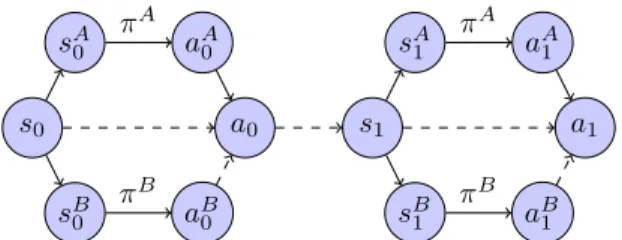
The intuition is that, when we do not know a∗ = π∗(s), we should maximize the agreement between aA =πA(sA)andB =πB(sB). In the first project (Section 6.1), we learn to estimate a safety cost called Approximate Clearance Assessment (ACE) (Otsu et al., 2020) which is used in the Enhanced Navigation (ENav) library (Toupet et al ., 2020). to plan paths for the Persistence Rover on the Mars 2020 mission (Williford et al., 2018).
Learning to Search with Retrospective Imitation
Introduction
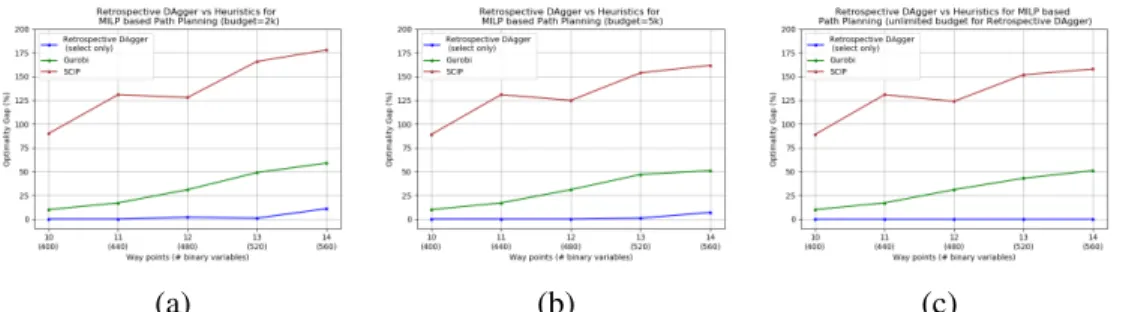
First, our approach is iteratively refined toward solutions that may be of better quality or easier to find from the policy than the original demonstrations. We demonstrate that our approach improves upon previous imitation learning work (He, Daume III, & Eisner, 2014) as well as commercial solutions such as Gurobi (for integer programs).
Problem Setting & Preliminaries
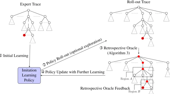
An imitation learning policy is initialized based on expert traces and is deployed to generate its own traces. The policy is then updated based on the feedback generated by the retrospective oracle, as shown in Figure 3.2.
Retrospective Imitation Learning
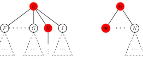
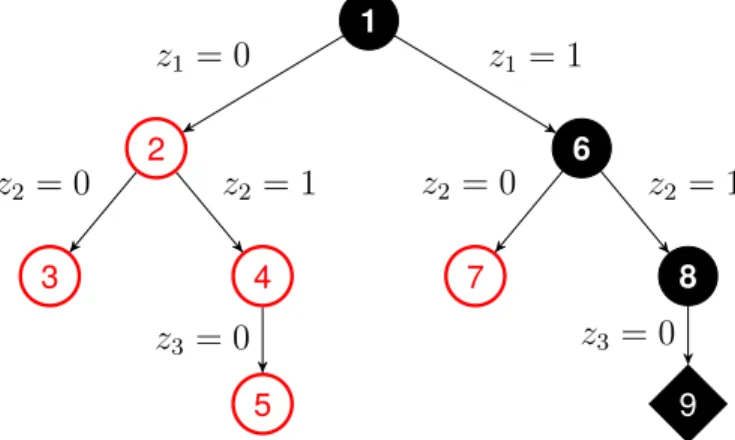
A retrospective oracle (with query access to the environment) takes a search track τ as input and outputs a retrospective optimal track π∗(τ, s) for each terminal states. In Figure 3.1, given the current track with a terminal state?(step 2O), the retrospective optimal track is the path along red nodes (step 3O).
Theoretical Results
Moreover, the retrospective feedback of the oracle fits the true training goal, while the dataset collected by imitation learning does not, as explained in Section 3.3. We then analyze how lower error rates affect the number of actions to reach the final state.
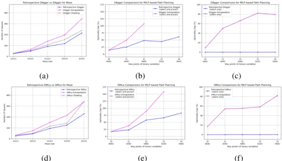
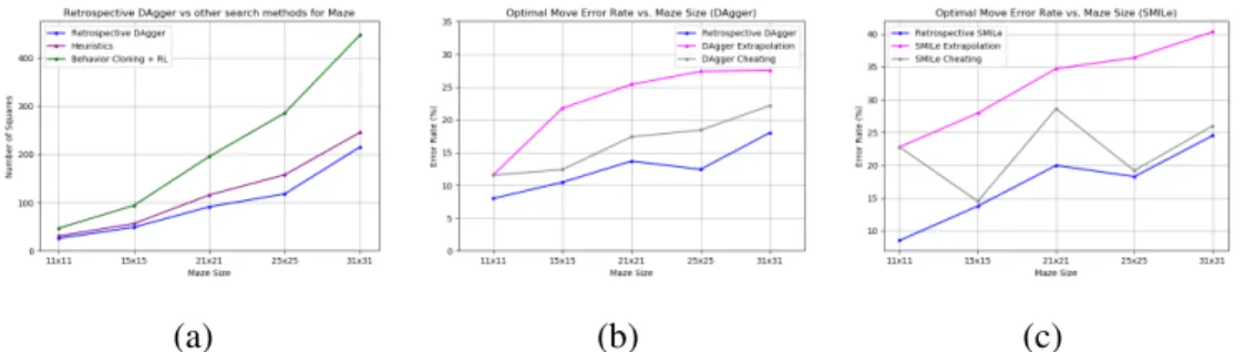
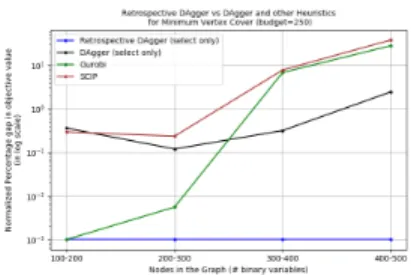
Experimental Results
The number of candidate repairs is potentially exponential in the size of the neighborhood, which explains the "big" in LNS. Maximizing Sequential Information: When Is Greed Near Optimal?” In: Conference on Learning Theory, pp.

Co-training for Policy Learning
Introduction
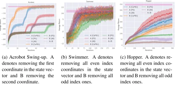
This is related to the conjoint training problem (Blum and Mitchell, 1998), where different representations of features of the same problem enable more efficient learning than using only one representation (Wan, 2009; Kumar and Daumé, 2011). In this paper, we propose CoPiEr (co-training for policy learning), a policy co-creation meta-framework that can include both reinforcement learning and imitation learning as subroutines.
Background & Preliminaries
A deterministic transition function is the obvious choice of adding a node to the current partial solution. A deterministic transition function is an obvious choice to add a new node to the search tree.
A Theory of Policy Co-training
For each state, we can directly compare the actions chosen by the two policies since the action space is the same. This insight leads to a more robust analysis result where we can narrow the gap between a co-trained policy and an optimal policy.
The CoPiEr Algorithm
For the special case with a shared action space, we can collect more informative feedback beyond the trajectory level. Instead, we collect interactive state-level feedback, as is popular in imitation learning algorithms such as DAgger (Stéphane Ross, Gordon, & D. Bagnell, 2011) and related approaches W .
Experiments
For example, Table 5.6 shows a benchmark comparison between Gurobi and a more state-of-the-art learning approach built on SCIP (Gasse et al., 2019) (reporting the geometric mean 1-shifted wall clock time on hard cases in their paper). Gross Margin Methods for Structured and Interdependent Production Variables.” In:Journal of Machine Learning Research6.9.
Incorporating Existing Solvers as Sub-routines
A General Large Neighborhood Search Framework for Solving Inte-
Designing algorithms for solving difficult combinatorial optimization problems remains a valuable and challenging task. Motivated by the aforementioned drawbacks, we study how to design abstractions of large-scale combinatorial optimization problems that can exploit existing state-of-the-art solvers as a generic black-box subroutine.
Background on LNS
At a high level, our LNS framework operates on an ILP by defining the decomposition of its full variables into disjoint subsets. We first describe a version of LNS for integer programs based on integer variable decomposition, which is a modified version of the evolutionary approach proposed in Rothberg, 2007, described in Alg 10.
Learning a Decomposition
The (weighted) adjacency matrix of the graph contains all the information to define the optimization problem by using it as input to the training model. Whichever characterization we use, the function matrix has the same number of rows as the number of integer variables we consider, so we can easily add the value of the variable to the solution as an additional function.
Emprical Validation for Learning-based LNS
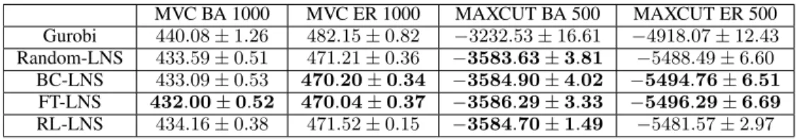
More importantly, in Figure 5.2d, Gurobi was given 2 hours of wall clock time and failed to match the solution found by Random-LNS in just under 5 seconds (time axis is in log scale) . In all three cases, the imitation learning methods, BC-LNS and FT-LNS, outperform Random-LNS.
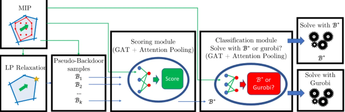
Learning Pseudo-backdoors for Mixed Integer Programs
We represent MIPs as bipartite graphs with different node characteristics for variables and constraints as in (Gasse et al., 2019), and use graph attention networks (Veličković et al., 2018) with pooling to learn both models.
Problem Statement for Learning Pseudo-backdoors
Learning Pseudo-Backdoors
These candidate pseudo-backdoor sets are ranked according to the scoring module S(P,B;θS) to predict the best pseudo-backdoorB∗. We then label the MIP instance and the pseudo-backdoor based on whether the pseudo-backdoor results in faster resolution time.
Experiment Results for Learning Pseudo-backdoors
We provide a thorough analysis of the proposed algorithm and prove strong performance guarantees for the learned target. We first consider the bound on the loss of the learned policy as measured against the expert's policy.

Learning Surrogates for Optimization
Learning Safety Surrogate for the Perseverance Rover
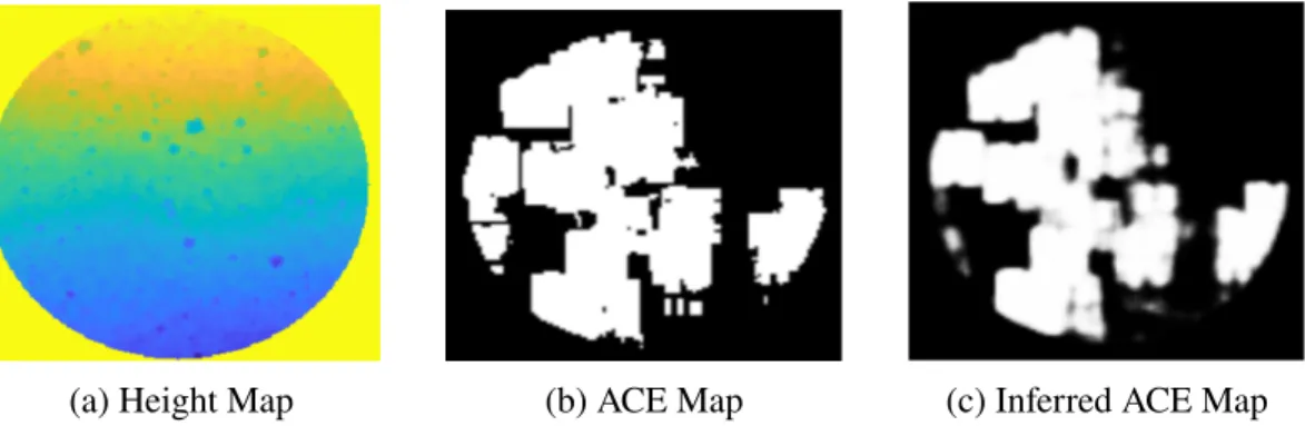
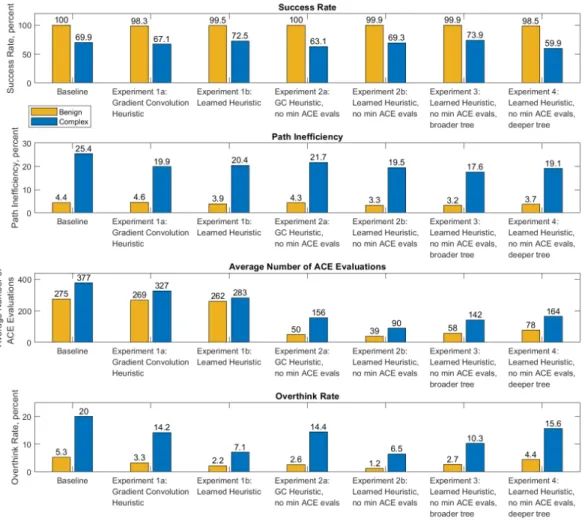
ENav uses the Approximate Clearance Evaluation (ACE) algorithm Otsu et al., 2020 to evaluate a sorted list of paths for safe passage. In this project, we train a machine learning (ML) classifier to derive ACE values to more efficiently sort the rover paths before the ACE evaluation step.
Method for Learning Safety Surrogate
However, the ACE cost depends not only on the terrain, but also on the rover's heading. Note that the result of this prediction is the probability that ACE returns a security violation, which is different from the output of the ACE algorithm itself.
Evaluations of the Learned Safety Surrogate
When the number of ACE estimates exceeds the threshold, this indicates that ENav is "thinking too much" and the rover may need to stop driving until a solution is found. This would result in far fewer times where the rover has to stop moving before the next path is found.
Learning Surrogate with Submodular-Norm Regularization
The last two properties allow us to prove approximation guarantees for the resulting greedy heuristic. Our results suggest that, compared to standard learning-based baselines: (a) LeaSuRe requires significantly fewer oracle calls during training to learn the target target (i.e., to minimize the approximation error against the oracle target); and (b) during the test, LeaSuRe achieves superior performance on the corresponding optimization task (i.e. to minimize the regret of the original combinatorial optimization task).
Background and Problem Statement
As we discussed in the previous sections, many sequential decision-making problems can be characterized as a restricted monotonic submodular maximization problem. For example, in the case of active learning, geexp(A, e) could be the expert acquisition function that ranks the importance of labeling each unlabeled point, given the currently labeled subset.
Learning with Submodular Regularization
In the cover set case, gexp(A, e) can be the function that scores each vertex and determines the next best vertex to add to the cover set. Then g can learn not only from the experts' selections of hA, xi, but can also see the labels of tuples that the expert would not have chosen.
Analysis for LeaSuRe
Note that the previous term regret corresponds to the average difference in score function between the learned policy and the expert policy. Although this result shows that LeaSuRe is consistent with the expert, it does not directly address how well the learned policy performs in terms of the utility obtained.
Evaluations LeaSuRe on Protein Engineering
Conclusion & Future Directions
Proofs
Since we have trajectory mappings between MA and MB, we can convert an occupancy metric in MA to one in MB by mapping each trajectory and running the count in the new MDP representation. So we can make this weaker assumption, which is also more intuitive and the original statement still holds with a different term.
Pictorial Representation of the Two-views in Risk-aware Path Planning107
For the MILP view, we directly use randomly generated rectangles to define the constraint space. However, for the QCQP view, we enclose the rectangular obstacles with a circle to define the quadratic constraint.
Discrete/Continuous Control Results in Tabular Form
Algorithm Configuration Results
Visualization
Each subimage contains information about the locations of obstacles (light blue squares) and the locations of waypoints after the current LNS iteration. We highlight the subset of 5 obstacles (red circles) and 5 waypoints (dark blue squares) that appear most often in the first neighborhood of the current breakdown.
Model Architecture
Barriers in red and transition points in dark blue are the most frequent in subsets leading to high local enhancement.
Domain Heuristics
The first is greedy: at each step, we accept the highest bid among the remaining bids, remove its desired items, and eliminate other bids that want any of the removed items.
Proof for section 6.7
Supplemental Details for the Protein Engineering Experiments