This thesis describes work towards the development of second generation laser interferometric gravitational wave detectors. Advanced LIGO is expected to make regular detections and open up the field of gravitational wave astronomy.
Gravity
Given the matter/energy distribution, the Einstein field equations are solved to find the gαβ metric that summarizes the spacetime geometry. Recent advances in numerical relativity, where the Einstein field equation is solved computationally using numerical methods, have led to rapid growth in our understanding of general relativity and the dynamical behavior of a system with strong gravity.
Gravitational Waves
The Evidence: PSR B1913+16
The most compelling, if indirect, evidence for the existence of gravitational waves comes from the binary pulsar system PSR B1913+16. It is deduced that the binary system loses energy because it emits the gravitational radiation predicted by general relativity.
Sources of Gravitational Waves and Detection Strategies
- The Stochastic Background of Graviational Radiation
- Continuous Wave Sources
- Compact Binary Coalesences
- Unmodeled Short-Duration Sources
As objects are inspired, the orbital period decreases, with a corresponding increase in the frequency of the emitted gravitational radiation. The detection strategy for such a signal relies on accurate waveform modeling combined with matched filtering of the data stream [24].
Gravitational Wave Detection
Terrestrial Gravitational Wave Detectors
- Resonant Mass Antenna
- Optical Interferometers
These antennas were solid masses that would essentially ring like a bell when a gravitational wave passed through them, temporarily pressurizing the mass. Saulson's book [34] provides an excellent introductory overview of the techniques involved in using interferometers as gravitational wave detectors.
LIGO
The LIGO Scientific Collaboration
A New Window on the Universe
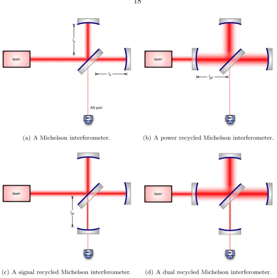
We can see how an interferometer can be used as a gravitational wave detector by recording the total accumulated phase of a light beam traveling between two freely falling masses separated by L, given by the integral of the spacetime metric along the way. Several configurations of interferometers that can be used as gravitational wave detectors are discussed in this chapter.
Noise
Quantum noise is solely due to quantum effects of the light in the interferometer and not due to any quantum mechanical motion of the test masses themselves [41]. Coupling of environmental noise to the interferometer is mostly due to acoustic disturbances of the sensor systems at the output port rather than the test masses themselves.
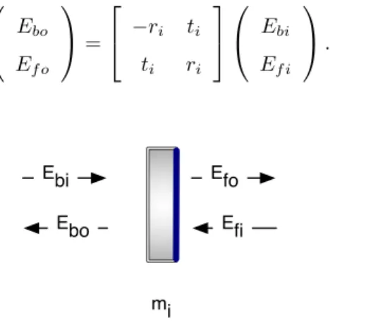
Mathematical Notations for Mirrors, Fields, and Spaces
We will decompose the spaces between the mirrors into macroscopic and microscopic lengths, where the macroscopic length is always an integer of the laser wavelength λ and the microscopic length is residual. The mirror operator in equation (3.9) and the propagation operator in equation (3.5) are enough to determine the static (equilibrium) response of an arbitrary interferometer configuration—all that is required is to use these operators to write down all field relations and solve the resulting system of coupled linear equations.
The Michelson Interferometer as a Gravitational Wave Detector
We lose sensitivity to the × polarized waves, which only excite the common mode, but gain immunity to light source noise—a valuable trade-off. Increasing the reinforcement for a given strain can be achieved by either increasing the length of the arms (cf.
Signal Extraction
Optical Heterodyne Detection
- Schnupp Asymmetry for Michelson Length Sensing
We can consider the case where we have audio sidebands on the carrier field and on the RF sideband fields we use as a local oscillator. We can transfer the RF sidebands to the asymmetric port of a Michelson interferometer using a Schnupp asymmetry [46], which is a macroscopic length difference between the arms of the Michelson.
Optical Homodyne Detection
However, if the arms are unequal in length (l− 6= 0), the asymmetric gate will actually be dark only at those wavelengths for which φ− = nπ. We can recover a linear detection function for the Michelson displacement by using this transmitted pair of RF sideband fields as a local oscillator in an RF heterodyne detection scheme.
Fabry-P´erot Cavities
Cavity Spatial Modes
A lens (or mirror) with focal length def (mirror curvature R= 2f) in the beam path changes the beam parameter according to The cavity waist is the smallest spot size of this eigenmode and it occurs directly.
Transfer Functions of a Fabry-P´erot Cavity
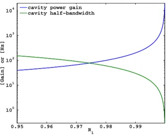
Here, ν0 is the cavity-free spectral region, q is the longitudinal number of modes (not the beam parameter), and R is the specular radius of curvature. Given that there is no cavity (i.e. just the end mirror without the input mirror), the cavity gain for a gravitational wave at ωac/2Lis.
The Pound-Drever-Hall Technique
The beam is modulated by an electro-optical modulator (Pockels cell), passes through a Faraday isolator (which separates the front beam from the back beam) and is the entrance to the cavity. When the cavity goes through resonance, the output of the mixer (and an invisible low-pass filter) is an error signal that goes through zero at resonance.
Adding Fabry-P´erot Cavities to the Arms of a Michelson Interferometer
Which RF sideband resonates (upper or lower) can then be selected using the Q-phase signal as a trigger, as it has a different sign for each of the two sidebands. Note that these concepts of symmetric mode and asymmetric mode only apply to signal (or noise) sidebands - carrier field power accumulation is of course the same in both modes.
Coupled Cavities
Antiresonant Short Cavity
Because at resonance for the wing cavity rc is opposite in sign to ri (so rc is positive), this actually represents the configuration with maximum power accumulation in the recycle cavity, and thus also in the wing cavity (since the power in the short cavity is effectively the input power to the arm cavity). The presence of sc in the numerator represents a zero in this transfer function at the arm cavity pole frequency; physically, the sidebands above this frequency are.
Resonant Short Cavity
For a source field in the arm cavity, there is no zero at the arm cavity pole frequency; rather, it will appear at the pole frequency of the short cavity.
Detuned Short Cavity
A particular effect of this RF sideband imbalance is a reduction in the cancellation efficiency for some noise on the sidebands, due to the different amplitudes on the upper and lower sidebands. This complicates the derivation of coupled system frequency responses, because now, instead of considering just the fields in the interferometer at a single frequency, we must consider two frequencies (±ωa) and the mirrors simultaneously; the resulting algebra becomes so tricky that it becomes easier for analytical work to work in the two-photon formalism.
Recycling
Power Recycling
For a given interferometer size (cavity length), the DC voltage signal transduction gain can be increased by increasing the power circulating in the arm cavities, which can be achieved in three ways: (1) using a more powerful laser; (2) increasing energy recycling profits; (3) increasing the DC gain in the arm cavities. The third option, increasing the DC gain in the arm cavities will reduce the detector bandwidth.
Signal Recycling
Since neither the absorption nor the laser power is uniform across the substrate, this will result in a temperature gradient in the substrate and an optical distortion given by the change in refractive index with temperature (dn/dT). This distortion will cause the substrate to act as a lens, distorting the wavefronts in the interferometer in a way that is detrimental to the sensitivity.
Resonant Sideband Extraction
Detuned RSE
- Two-Photon Formalism
- The RSE Response Function
- Detuned RSE Interferometers as Optical Springs
- Dynamical Instability
- Anti-spring
- The Detuned Resonant Sideband Extraction Interferometer with Power Recy-
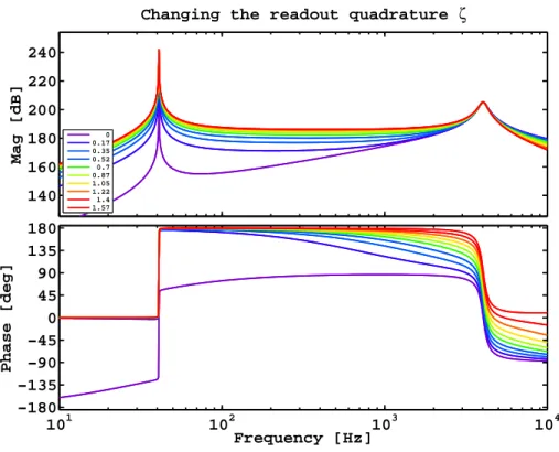
The optical resonance is just the one described in section 3.8.3 and shown in figure 3.8(b): the coupled cavity system is detuned from a zero-frequency resonance. As the signal recovery cavity goes from resonant to the carrier (brown) to anti-resonant to the carrier (violet), the bandwidth of the detector increases at a cost of overall gain.
Feedback Control
Noise reduction
The effect of these noises can be reduced by eliminating the noise source, reducing the coupling of the noise to the DARM, or suppressing the noise with feedback. Almost all of the significant infrastructure at LIGO is devoted to at least one of these three techniques.
Transduction linearity
The first, reduction of noise, concerns all aspects of the system that contribute to the detection (seismic isolation, suspensions, interferometric DOFs other than DARM, angular DOFs, etc.). These noises can be coupled into DARM by various mechanisms, and they will mask a gravitational wave signal.
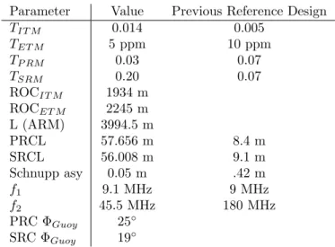
The Advanced LIGO Design
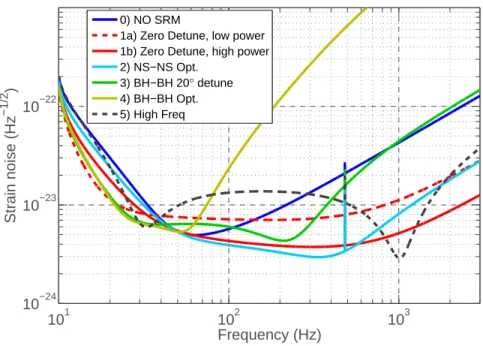
The other curves can all be achieved by changing a combination of the detuning phase and the input power. The carrier and modulation sidebands experience different resonant conditions in different subsections of the interferometer; this is the resonance profile (more in chapter 6).
DC Readout
This means that the RF sidebands do not undergo any significant filtering from sidebands or scc, and any modulation sideband noise (either from the laser itself or the modulator) thus passes essentially unchanged into the interferometer's detection port. Once there, amplitude and phase noise on the modulation sidebands can contaminate the signal when these sidebands are used as a local oscillator (cf.
Considerations
- Laser Noise Couplings
- Spatial Overlap
- Output Mode Cleaner
- OMC noise mechanisms
- Oscillator Noise
- Oscillator amplitude noise
- Oscillator phase noise
- Flicker Noise
- Unsuppressed Signal
- Shot Noise
- Signal Linearity
The noise on the carrier is filtered in the interferometer and couples to the asymmetric gate via interferometer asymmetries (particularly mismatches in the arm cavity parameters). Because in DC readout, both the local oscillator and the signal come from the same place (that is, the arm cavities of the interferometer), they are in the same transverse spatial mode and thus have perfect spatial overlap at the photodetector.
Decision
The main task of the 40m is to act as a control and configuration prototype; 40 m is not a noisy prototype. Currently, the primary task of 40 m is to study the length detection and control scheme for Advanced LIGO.
Vacuum and Seismic Isolation
Suspensions
The combined coil and shade sensor is called OSEM (Optical Sensor and Electromagnetic Actuator); The OSEMs are fixed to the suspension cage. Local damping only dampens the pendulum resonance, with a bandwidth of ∼2 Hz, to reduce the effect of noise in the shadow sensor above this frequency from the imposition on the optical motion by the control system.
Electronics and Digital Controls
The suspension is controlled by the digital suspension controller (DSC), which will be described in section 5.4. The OMC computer then transmits this signal via a fiber network, it is filtered to the LSC computer and the control signal is sent to the digital suspension controller via fiber.
Pre-Stabilized Laser
- MOPA
- Power Stabilization
- Frequency Stabilization
- Pre-Mode Cleaner
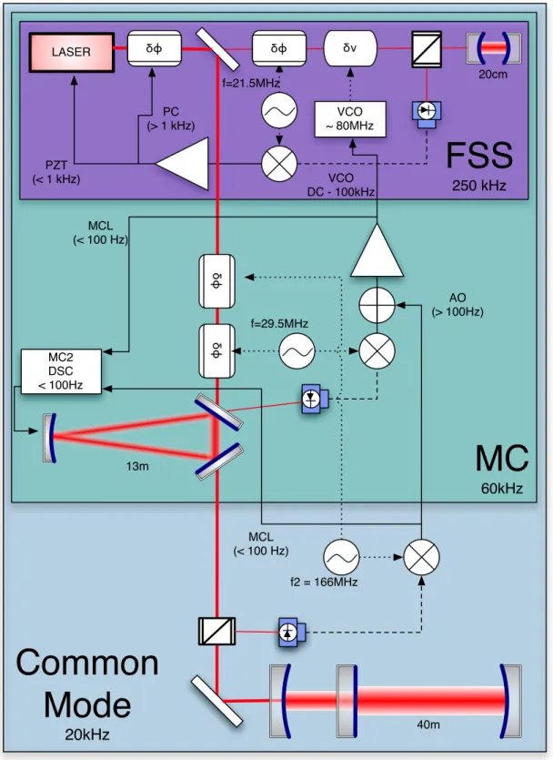
The FSS stabilizes the laser frequency to a frequency reference cavity (RC,F ~9500) a standard PDH setup, with the primary actuator a Pockels cell (PC) at the output of the MOPA, up to a bandwidth of 250 kHz ( although the system is designed for 500kHz). By applying a voltage to the VCO, the laser frequency can be shifted while the RC remains exactly at resonance.
Input Optics
Phase Modulations
- A Mach-Zehnder interferometer for non-cascaded RF sidebands
The FSS can then be used as a frequency actuator, limited by the FSS bandwidth, and with a range determined by the limits of the VCO (±7 MHz) rather than the linewidth of the RC (~76 kHz) ). The resulting 'modulation depth' is a factor of 2 lower at the output of the MZ than in the arm.
Input Mode Cleaner
This second set of sidebands appears, relative to the carrier frequency, at the difference frequency between the two sidebands. To avoid this, the phase modulation sidebands are applied in parallel, in the arms of a Mach-Zehnder interferometer.
Input Isolation, Mode Matching, and Steering
These sidebands-on-sidebands corrupt the purity of the DDM signals, making them highly affected by carrier light, and thus less useful in isolating the short degrees of freedom of motion in the long degrees of freedom [76].
The Common Mode Servo
Interferometer
Output Optics
- Output Mode Cleaner
- OMC Length Sensing and Control
- Output Steering
- Output Mode Matching
- Higher Order Mode Content at Asymmetric Port
- Photodetectors
It is a 4:1 beam reduction telescope designed to match the beam circulating in the interferometer (banded at ITM) to the OMC cavity mode. The recombination of the two beams in the Michelson then approximates the mode of signal transmission.
The Future
About 3% of the power in this beam is contained in RF sidebands, which are immediately reflected by the arms and transmitted by the Michelson, so this establishes the lower limit of the mode matching. This chapter completes the picture by describing how to sense the other longitudinal degrees of freedom and how we control them all, focusing on the specific LSC scheme of 40 m (already described in Chapter 5).
Principle
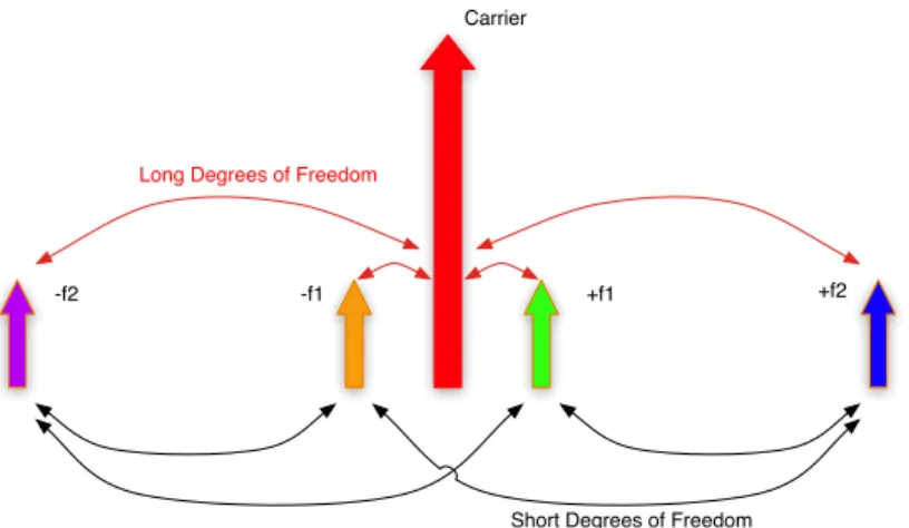
The 40 m LSC configuration is designed to test a potential configuration for Advanced LIGO, specifically a detuned RSE interferometer. The resonance profile of these five frequencies can be seen in Figure 6.1(b) and is described in Section 6.2.
Resonance Profile
This should be more sophisticated, especially to feel the SRCL degrees of freedom. The carrier plus two pairs of non-cascaded phase modulation sidebands can be represented as five incident light frequencies in the interferometer (cf.
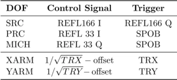
Sensing
- Signal Selection: Ports, Frequencies, and Quadratures
- Double Demodulation
- Sideband Imbalance and Offsets
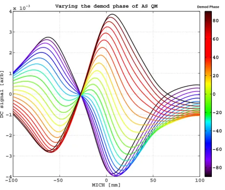
- Measuring Demodulation Phases
- Configuration Space and the Operating Point
- Discriminants
- Frequency dependence
- Position dependence
- Example matrix at operating point
- SPOB
- Non-resonant sideband
Moreover, all the elements are non-linear functions of the microscopic positions of each optic in the interferometer (ie the location in configuration space) and will also vary with the sound frequency ωa. In general, each element of the sensing matrix is a non-linear function of the position of all the interferometer optics.
Control
Matrices and Bases
- Input Matrix
Ensuring that the control basis is exactly the canonical basis requires accurate calibration of the mirror actuators; this is not difficult for ETMs (it is part of the calibration procedure in Chapter 7). The second reason that the control base is different from the canonical base has to do with lock acquisition (more on that in Chapter 8).
Feedforward Corrections
In an ideal system, the input matrix would be the inverse of the detection matrix M; then the error signals for the control loops would be sensitive only to motion of their own degrees of freedom. The measurement and inversion of the input matrix (the part that connects the DDM signals to these DOFs) is performed during the lock acquisition bootstrapping, described in section 8.5.
Discussion
- Free Swinging Michelson
- ITM Calibration
- ETM Calibration
- DARM calibration
- Tracking
- Comment
Here we are only concerned with the calibration of the DARM error signal in the frequency domain. With the interferometer optics aligned to create a simple Michelson, excite the optics lengthwise and measure the peak-to-peak amplitude of the signal as the Michelson oscillates through the entire fringes.
Calibrating the 40 m Detuned RSE Interferometer
- Actuator Calibration
- DARM Calibration
- Modeling
- Tracking
Part of the work of the LIGO Scientific Collaboration Detector Calibration Subgroup is also to understand in detail all the smaller parts of the model (ie the ADCs considered individually, the coil drivers, etc.) and make sure the parts fit together correctly. Assuming that Metm really behaves like a pendulum at the frequencies where radiation pressure matters (below 100 Hz) should not be controversial; it's the behavior of the actuators (ie the OSEMs) that really matters, and that's mainly above a kHz.
Calibration for Advanced LIGO
The one at 3.8kHz is believed to be in the piezo actuated input control mirrors, but this has not been confirmed. The peaks at 3.8 kHz mask the resonance in the DARM response at this frequency that might otherwise be visible.
Lock Acquisition: The Path to Control
The test masses (and many other auxiliary optics) in an interferometer are suspended; in the absence of control, they move in µm levels and therefore the fields in the interferometer change rapidly and unpredictably. Lock acquisition is the process of bringing the interferometer from the uncontrolled state to the controlled operating point.
Lock Acquisition of a Resonant Cavity
- Threshold velocity
- Normalized PDH locking
- Loop Triggering
- Offset locking
When the transmitted power exceeds a certain threshold, indicating that the cavity is close to resonance, the control turns on. This technique is very suitable for locking the cavity at a point where the power build-up is half of the maximum.
Lock Acquisition of Coupled Cavities
Lock Acquisition for Initial LIGO and Virgo
Virgo also initially implemented the LIGO protocol of dynamic matrix inversion, but then decided on the variable finesse technique ([91]), which is in a sense a different philosophy: control is initially obtained in place in configuration space that is not the operating point. of the interferometer, and the interferometer is then brought to its operating point while under control. The Michelson offset is then reduced in a controlled manner along with the PRM alignment until the interferometer is at its operating point.
Lock Acquisition of a Detuned Resonant Sideband Extraction Interferometer with
Bootstrapping
Interferometer subsets
Alignment
Double Demodulation signals
The Lock Acquisition Procedure for the Caltech 40 m Interferometer
- Initial Acquisition
- The spring and the anti-spring
- Locking the spring and the anti-spring
- The Protocol
- Adaptive compensation filter: the moving zero
- Other Protocols
- Scripting Tools
This signal is fed back to the laser frequency (obviously after AC coupling) to the AO path of the CM servo. As the CARM offset is reduced, the tuning of the CARM degrees of freedom changes, causing a change in the optical facility.
Deterministic Locking
The Future: It’s easy being green
- Envisioned lock acquisition procedure
- Advantages of this technique
- Alternative Technique
The resulting green light can then be locked into the arm cavity in the same way, with the fault point of the phase-locked loop now taking the place of the frequency actuator. The feedback to the error point of the phase-locked loop is now the arm cavity length detection signal; it can be used in the same way to dampen the arm cavity with speed.
Discussion
Noise Injections
- Laser Amplitude Noise
- Laser Frequency Noise
- Oscillator Noise
The simulation includes only 6 servo loops and the configuration does not change during the course of the swept sine calculation. The noise coupling was measured in this case by injecting a signal into the error point of the common-mode Servo (see section 5.7), causing a frequency mismatch between the laser light and the CARM degrees of freedom; the signal was then coherently demodulated into the gravitational wave channel to determine the transfer function.
Power Recycled Fabry-P´erot Michelson Interferometer
- Simulation
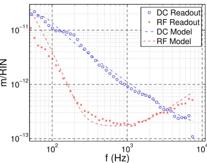
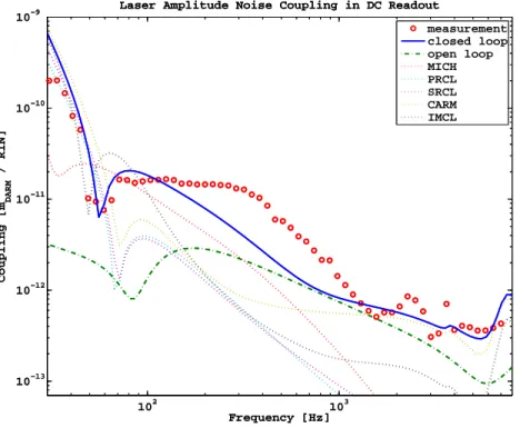
- Laser Amplitude Noise
- DC Readout
- RF Readout
- Laser Frequency Noise
- Oscillator Phase Noise
- Oscillator Amplitude Noise
An IFR2023A signal generator is used as the source signal for the RF modulation sidebands on the laser light, and the same oscillator signal is then used in demodulating the signal. In the DC readout scheme, the RF modulation sidebands are used for sensing and controlling auxiliary degrees of freedom, and so noise on these sidebands can couple indirectly to DARM.
Detuned RSE Interferometer
- Length Offsets
- Cyclical dependencies
- Mode cleaner length
- Effect on DARM calibration
- Simulation
- Feedback and Offsets
- The simulated noise traces
- Effects not included
- Auxiliary loop coupling
- Laser Amplitude Noise
- DC Readout
- RF Readout
- Laser Frequency Noise
- DC Readout
- RF Readout
- Oscillator Phase Noise
- DC Readout f 1
- DC Readout f 2
- RF Readout f 1
- RF Readout f 2
- Oscillator Amplitude Noise
- DC Readout f 1
- DC Readout f 2
- RF Readout f 1
- RF Readout f 2
The simulated links shown fit the data perfectly: the simulation is much too slow for an automated adjustment mechanism. The main coupling path is similar to an energy-recycled interferometer; fluctuations in the input power reach the signal cavity (that is, the asymmetric side of the beamsplitter) in the same way, but the signal recycling cavity then re-injects these fluctuations in the asymmetric mode (with a quadrature rotation).
Conclusions
This chapter describes a search for gravitational waves using data from the fifth LIGO science run, which took place between 1 December 2005 and 30 September 2007. These results use data from the LIGO detectors, but have not been reviewed or endorsed by, and do not represent the scientific opinion of, the LIGO Scientific Collaboration.
Stochastic Gravitational Waves
This chapter presents results using the radiometer technique on data from LIGO's fifth science suite, which was much longer and more sensitive than S4. In particular, we target Sco-X1, the nearest 15 globular clusters and the galactic center, which are promising locations for containing multiple, faint, superimposed and unmodeled sources.
Detecting stochastic gravitational waves
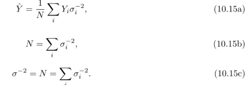
- Isotropic strategy
- Segmenting Data and Optimal Combination
- Gravitational Wave Radiometry
- The Point Spread Function
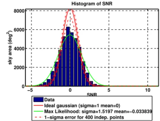
The detailed structure of the PSF will vary with sky position and frequency of the source. This means the resolution of the radiometer is limited to something of order ~ 400 independent points in the sky, a number estimated in [71].
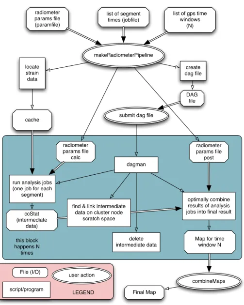
Analysis Pipeline
Because the radiometer algorithm depends on lateral variations in antenna reception to provide directional discrimination, in theory the PSF should not change with right elevation of the source, although it will with declination. A lower limit can be placed on the magnitude of the point spread function by assuming limited detection of gravitational wave diffraction, which limits the resolving power of an instrument of known formula.
Limits on Gravitational Waves
- Detection
- The Data
- Data Quality
- Frequency Masking
- Delta-Sigma Cut
- Posterior Distributions and Upper Limits
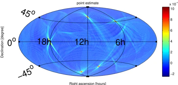
- Gravitational Wave SkyMap
- Injection
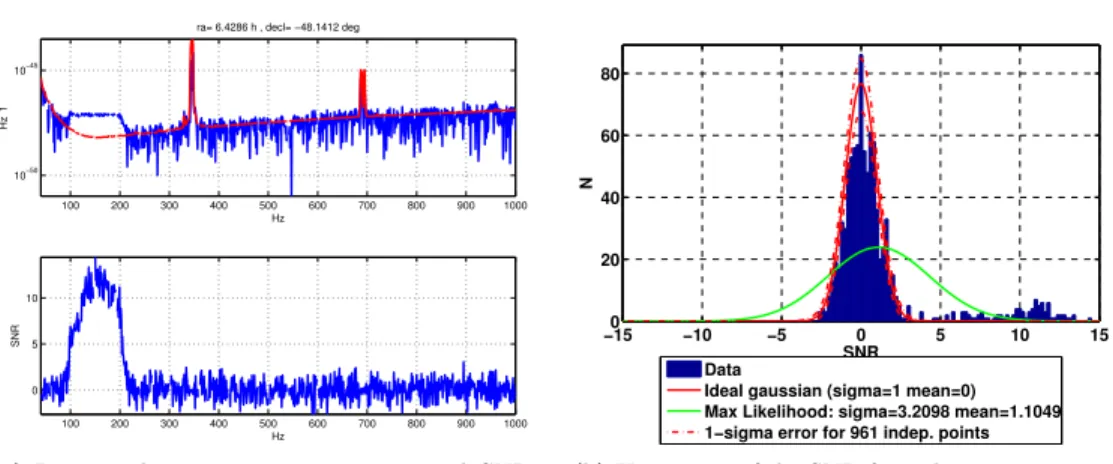
For the radiometer search, this eliminates 36×0.25 Hz bins, which is about 0.05% of the total bandwidth. It is clearly visible as a dominant hot spot. a) SNR map of S5 runs for a flat source strain spectrum.
Frequency and Location Resolved Searches
- Upper Limit on gravitational waves from Sco X1
- The Galactic Center
- Globular Clusters
- Untargeted Narrowband Search on the Whole Sky
- Injection
The upper bound in Figure 10.8 has used the corresponding result from the S4 run [106] as Bayesian prior (see section 10.4.4); the new limit exceeds the previous result by a factor of about 5. This situation is similar to that of the galactic center. a) Upper limit (90% confidence level) for voltage from the galactic center.
Future Work
- Detection Thresholding
- Multi-baseline Radiometry
- Transient Searches
- Clustering
In (a, bottom), the SNR shows a clear clustering of high values at the injection frequencies. In (b), the histogram of SNR across frequency sets shows clear deviations from a standard normal distribution, with many outliers at high SNR.
Discussion
We developed the first lock-in acquisition protocol for a suspended mirror interferometer with five longitude degrees of freedom, a critical step in the development of second generation interferometric gravitational wave detectors. The 40 m prototype effort has made significant contributions to the advanced LIGO design effort and thus to the gravitational wave detection community.
Asymmetries and Couplings
Laser noise coupling to asymmetric port
Equilibrium Frequency Response
Coupled Cavities
Servo Stability
Bode gain-phase relationship
Conditional Stability
Servo Bandwidth
Feedback Filter Design
MIMO control
- Cross Coupling
FINESSE
GWINC
Optickle
Looptickle
E2E: End to End
FFT
MATLAB code
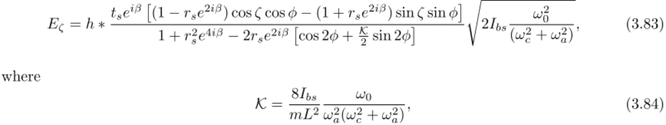
The RSE response function
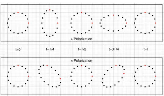
- Effect of a GW on a circle of test particles
- Input and output fields of a mirror mass
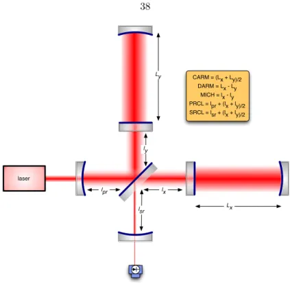
- Michelson based interferometer topologies for gravitational wave detection
- A Fabry-P´erot Cavity with overlapping waves
- Cavity gain vs. bandwidth
- A schematic of a typical PDH length sensing setup
- The PDH signals for a single cavity
- A three mirror coupled cavity
- Effect of adding a third mirror with a short cavity on the bandwidth of the coupled
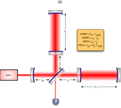
- A Power Recycled Fabry-P´erot Michelson Interferometer
- A Dual Recycled Fabry-P´erot Michelson Interferometer
- Changing the detuning of the signal cavity
- Frequency response in different readout quadratures
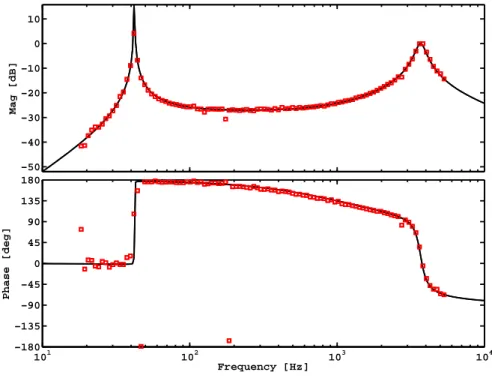
- Measurement of the opto-mechanical RSE response
- Measurement of the opto-mechanical RSE response in an anti-spring configuration
- Projected sensitivity for possible operating modes of Advanced LIGO
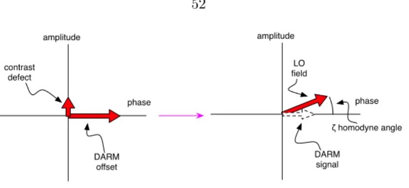
- Phasor diagram of the asymmetric port in an RF readout scheme
- Phasor diagram of the asymmetric port in a DC readout scheme
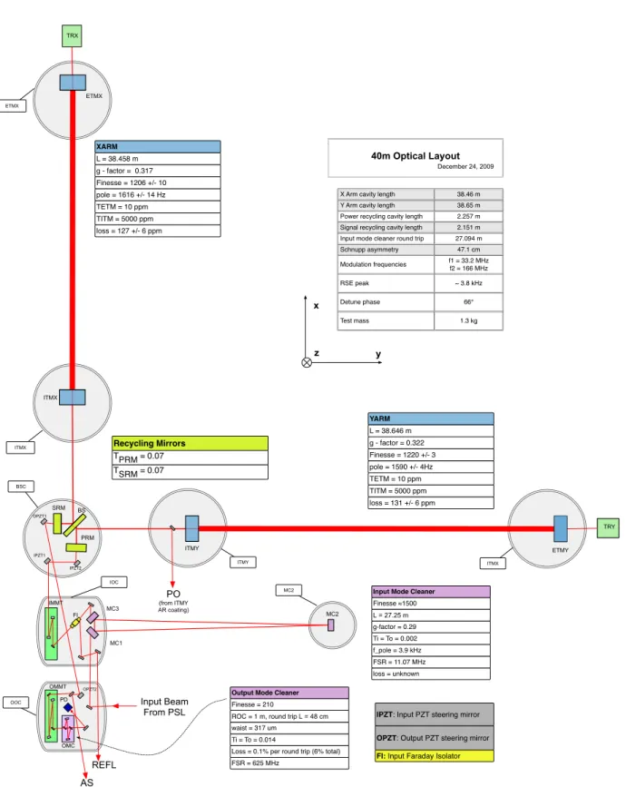
- The layout of the 40 m
- A MOS suspension
- Real time control network example
- The laser frequency stabilization system
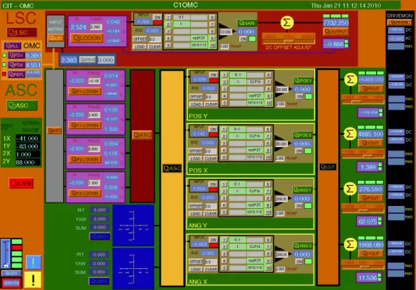
- An example EPICS control screen
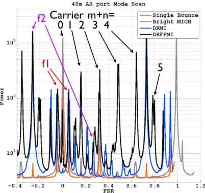
- Mode scans of the AS port
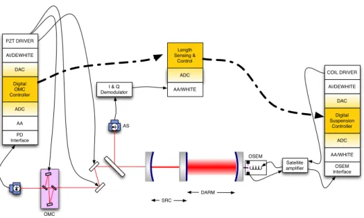
- The DC Readout sensing chain
- The length sensing and control scheme
- Demod phase errors will lead to offsets
- Modeled and measured response of a differential demodulation error signal
- Frequency dependent magnitude of the OMC DC row of the matrix of discriminants. 81
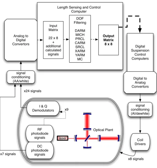
- Block diagram of length sensing and control system
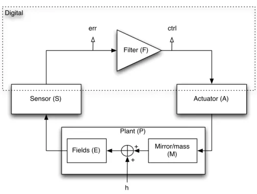
- Feedback loop block diagram
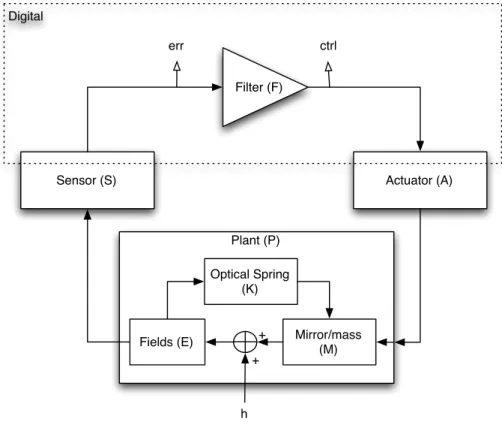
- Feedback loop block diagram
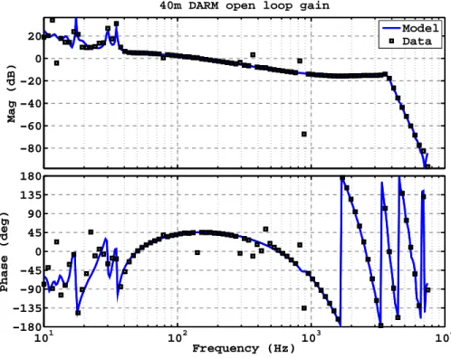
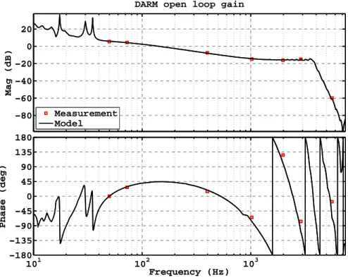
- An example DARM open loop transfer
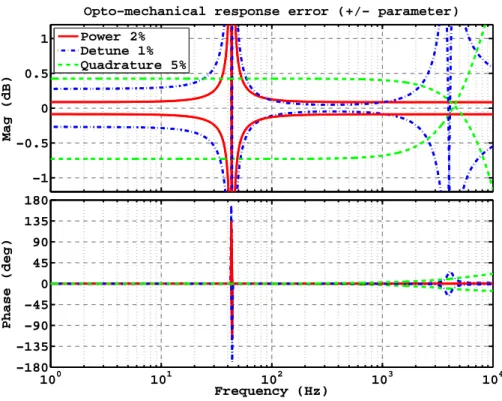
- Ratio of the opto-mechanical response to nominal with given parameter variation
- An example DARM open loop transfer
- DARM noise spectra for a detuned RSE interferometer
- Error signals for a single Fabry-P´erot cavity
- Signals and DOFs for bootstrapping
- A typical initial acquisition
- Histogram of waiting times to acquire initial control of five length degrees of freedom. 111
- DARM demodulation phase rotation
- The optical response (magnitude only) of the CARM DOF at several CARM offsets
- Interferometer power during lock acquisition
- dB magnitude of the CARM (sensed at) open-loop opto-mechanical frequency response 118
- Dynamic compensation filter used in the CARM loop
- CARM cavity response and open loop transfer functions
- The flow of the main watch script used for locking
- The hierarchcy of scripts
- Laser intensity noise coupling for the 40 m Fabry-P´erot Michelson interferometer with
- Laser frequency noise coupling for the 40 m Fabry-P´erot Michelson interferometer with
- Oscillator phase noise coupling for the 40 m Fabry-P´erot Michelson interferometer with
- Oscillator amplitude noise coupling for the 40 m Fabry-P´erot Michelson interferometer
- DC readout laser amplitude noise coupling
- RF readout laser amplitude noise coupling
- DC readout laser frequency noise coupling
- RF readout laser frequency noise coupling
- DC readout f 1 oscillator phase noise coupling
- DC readout f 2 oscillator phase noise coupling
- RF readout f 1 oscillator phase noise coupling
- RF readout f 2 oscillator phase noise coupling
- DC readout f 1 oscillator amplitude noise coupling
- DC readout f 2 oscillator amplitude noise coupling
- RF readout f 1 oscillator amplitude noise coupling
- RF readout f 2 oscillator amplitude noise coupling
- The estimate of the variance for each data segment is calculated using data from neigh-
- Radiometer point spread function
- The radiometer analysis
- The radiometer pipeline
- Representative strain noise curves from the 4 km LIGO detectors during the fifth LIGO
- Upper limit map from S5 run
- An injected broadband point source
- Limits on gravitational radiation from Sco-X1
- Limits on gravitational radiation from the galactic center
- Results from GC1
- Results from GC2
- Results from GC3
- Results from GC4
- Results from GC5
- Results from GC6
- Results from GC7
- Results from GC8
- Results from GC9
- Results from GC10
- Results from GC11
- Results from GC12
- Results from GC13
- Results from GC14
- Results from GC15
- Injected point source
Laser amplitude noise coupling paths in DC readout
Laser amplitude noise coupling paths in RF readout
Laser amplitude noise coupling in RF readout
Laser frequency noise coupling paths in DC readout
Laser frequency noise coupling paths in RF readout
Laser frequency noise coupling in RF readout
Indexed fields in a resonant cavity
Reflected and transmitted fields through a cavity
Schematic idealization of a canonical feedback loop
Example feedback loop