MICRO-PRICE DYNAMICS IN SMALL OPEN ECONOMIES:
LESSONS FROM ECUADOR
By Craig Benedict
Dissertation
Submitted to the Faculty of the Graduate School of Vanderbilt University
in partial fulfillment of the requirements for the degree of
DOCTOR OF PHILOSOPHY in
Economics January 31, 2019 Nashville, Tennessee
Approved:
Mario J. Crucini, Ph.D Kevin X.D. Huang, Ph.D.
Gregory W. Huffman, Ph.D.
Anthony Landry, Ph.D.
To my family
ACKNOWLEDGMENTS
I am extremely thankful to my advisor, Mario J. Crucini. Without his abundant guidance and patience, this dissertation would not be possible. There are only a handful of men in this world who could have walked me through the process and without him, I would truly have been lost. I have always known he was a man of considerable skill. Working with him the last several years has shown him to be a man of exemplary character as well.
I am also grateful to my committee members, Gregory Huffman, Kevin Huang, and Anthony Landry. Kevin and Greg’s guidance was invaluable in helping me navigate the pitfalls of graduate school and the job market. I still remember much of the advice they gave me in my first years in the program. I am also especially grateful to my co-author and friend, Anthony Landry, who always provided words of encouragement and set an excellent example for me as we worked on our paper together.
Last, but not least, I am forever indebted to my incredibly supportive family and friends, especially my parents, Craig and Diohn, for the stability they provided and the unwavering faith that pushed me to keep going. I thank my siblings and their spouses, Kelly, Ryan, Autumn, Rob, Kirk, and Molly, for their constant support. Lastly, I thank my friends who walked with me on this arduous journey, especially Nayana Bose and Zhongzhong Hu whose advice helped me to navigate the difficulties of grad school.
TABLE OF CONTENTS
Page
DEDICATION . . . ii
ACKNOWLEDGMENTS . . . iii
LIST OF TABLES . . . vi
LIST OF FIGURES . . . vii
1 Introduction . . . 1
2 On What States Do Prices Depend: Answers from Ecuador . . . 5
2.1 Introduction . . . 5
2.2 A Brief Monetary History of Ecuador . . . 8
2.2.1 The Data . . . 9
2.2.2 Three Inflation Regimes . . . 11
2.2.3 Price Changes in Ecuador . . . 13
2.3 The Model . . . 16
2.3.1 A Menu Cost Model of Price Adjustment . . . 16
2.3.2 Model’s Solution and Calibration . . . 19
2.4 Results . . . 22
2.4.1 Benchmark model . . . 22
2.4.1.1 Model with idiosyncratic import prices . . . 25
2.5 Conclusion . . . 27
Appendix A Distribution Shares . . . 30
Appendix B Equations, and Solution Method . . . 39
B.0.1 Profit function . . . 39
B.0.2 Solution Method . . . 39
Appendix C Model with variable markups . . . 41
3 The Law of One Price in Ecuador . . . 43
3.1 Introduction . . . 43
3.2 Unit Root Tests for LOP Convergence . . . 47
3.2.1 Persistence in LOP Deviations . . . 51
3.3 Compositional Bias . . . 57
3.3.1 Estimation . . . 62
3.3.2 Results . . . 63
3.4 Conclusion . . . 66
4 Exchange Rate Pass-through in Ecuadorian Cities . . . 67
4.1 Introduction . . . 67
4.2 The Geography of Ecuador . . . 69
4.2.1 Empirical Strategy . . . 71
4.2.2 Pass-through by Good . . . 74
4.2.3 Pass-through by Cities . . . 77
4.2.4 Pass-through and Distance from the Coast . . . 78
4.3 Conclusion . . . 79
Appendix D Pass-through Regression Results . . . 80
BIBLIOGRAPHY . . . 97
LIST OF TABLES
Table Page
2.1 Summary of Monthly Price Facts . . . 13
2.2 Stochastic Properties of Shocks . . . 20
3.1 ADF Unit Root Rejection Frequencies . . . 50
3.2 IPS Unit Root Rejection Frequencies . . . 52
3.3 Median Persistence Estimates . . . 54
3.4 Estimated parameters of the AR(1) model . . . 63
4.1 Ecuadorian Cities . . . 71
4.2 Pass-through into CPI . . . 73
4.3 Pass-through by city . . . 78
D.1 Pass-through by Goods . . . 80
D.2 Coastal Difference Regression . . . 88
LIST OF FIGURES
Figure Page
2.1 Monthly CPI Inflation in Ecuador by Regime . . . 12
2.2 Monthly Frequency of Price Adjustment in the Data . . . 15
2.3 Distribution of Import Price Volatility . . . 21
2.4 Costs Variance and Policy Functions . . . 23
2.5 Average Frequency of Price Adjustment by Regime, Data versus Model . . . 24
2.6 Frequencies of price adjustment by regime and distribution share . . . 26
2.7 Monthly Frequency of Price Adjustment in the Model . . . 28
C.1 Monthly Frequency of Price Adjustment in the Model with Variable Markups 42 3.1 Kernel Density for the Law of One Price Deviations . . . 54
3.2 Kernel Density of Persistence Estimates . . . 55
3.3 Kernel Density Cumulative Impulse Response Estimates . . . 56
3.4 Sectoral-mean first order autocorrelation estimates against sectoral distribu- tion shares . . . 58
3.5 Sectoral-mean CIR estimates against sectoral distribution shares . . . 59
3.6 ψiFunction . . . 64
4.1 Map of Ecuador . . . 70
4.2 Weighted Exchange Rate . . . 72
4.3 Nontraded Input Share versus Short-Run Pass-through . . . 76
4.4 Nontraded Input Share versus Long-Run Pass-through . . . 77
Chapter 1
Introduction
Prices have always been understood to have an important impact on the creation of goods and services, but the extent of that impact has swayed back and forth as the tides of economics have turned. At first glance, the nominal price should be nothing more than a number that can be changed arbitrarily without distortion in the production of goods and services. Adding a zero to the denomination of all ten dollar bills should leave the consumer in the exact same situation as he had been previously. However, since Keynes, these merely nominal changes in the price have been understood to have much longer and more meaningful impacts. As the birth of Keynes and macroeconomics was more than one hundred years ago, it would seem like there would be little left to be said about such a critical phenomenon. Nevertheless, the information age has exposed new questions as more precise data in the form of micro-prices has become available. The introduction of micro-price data has led to new analyses that contribute to understanding the connection between the nominal and the real. This study contributes to that tradition through a careful analysis of the movement of retail prices in three separate but equally important dimensions through the lens of one small but dynamic country with a fascinating monetary history.
Those dimensions are the frequency of price change, the relationship of prices to each other, and the reaction of prices to external shocks, in this case, a shock to the exchange rate.
While seemingly narrow in its subject, the use of a single, small, export-dependent country such as Ecuador serves as a case study for investigating much broader topics throughout both monetary economics and international finance. For example, the stick- iness of retail prices has large and lasting impacts on the neutrality of money, a subject covered in great detail with respect to the United States. By looking at the subject through
the lens of Ecuador, we can observe the magnitudes of and changes in variables that are not present in a US context. At no point in recent history has the developed world had inflation reach the levels as we see in in Ecuador nor has it stabilized so abruptly. By looking at the changes we can observe their impact more readily on the variables of interest to broaden our understanding of the factors in play. All three chapters are important not just because of the implications for Ecuador and developing nations but for the world as a whole. Ecuador is merely the magnifying glass we can use to shed light on prices throughout the world.
Chapter 2 investigates the movement of prices. The parameter of interest here is the frequency of price change and how this number relates to various conditions or states within the country of Ecuador. In this chapter, my co-authors and I demonstrate that prices in Ecuador have a structural pattern in the frequency of adjustment. As is true in all menu cost models, firms reprice more frequently in higher inflationary regimes, but we also see that goods that are more likely to reprice in a period of hyperinflation are also more likely to reprice in a period of stability brought about by dollarization. These patterns are robust across three vastly different macroeconomic regimes in Ecuador.
To explain this phenomenon, we create a menu cost model of price adjustment where firms import goods from competitive markets overseas and use labor to distribute final goods throughout the country. Using this model, we show that cost structure plays a critical role in explaining the frequency of price adjustment. Movements in the price of underlying components shift the costs of the firm and thus lead to more frequent repricing. As the traded component is much more volatile than the wage, our model predicts that goods that are more reliant on traded inputs will change their price more frequently than goods depen- dent on non-traded inputs such as labor. However, the model also predicts that goods more reliant on one component will also reprice more frequently than goods that use an equal combination of traded and non-traded inputs. Firms that use a diverse set of inputs can ad- just to cost shocks more easily by substituting production towards the cheaper input; they also benefit from the benefit of diversification to the extent inputs prices are imperfectly
correlated with each other.
Chapter 3 looks at prices and their relation to each other within Ecuador. Leaning on the prior literature relating to the purchasing power parity paradox and the law of one price, I present evidence strengthening the law of one price within the country of Ecuador. Using an Augmented Dickey-Fuller test and an Im et al. (2003) test for stationarity, I find a strong likelihood to reject the null hypothesis of a unit root. Furthermore, I estimate persistence of deviations in the law of price to be extremely low, with half-lives on the order months.
This suggests prices within Ecuador converge more quickly compared to other studies, especially those in developed nations.
In addition, Chapter 3 argues that because prices are a combination of both traded inputs and non-traded inputs, this leads to a phenomenon known in the literature as compositional bias where retail prices take on unit root properties of their non-traded input, even if the final good is considered tradable. Under the assumption of a Cobb-Douglas production function, I scrutinize the process of combining the components into one retail price. As- suming both inputs follow an AR(1) process and estimating parameters for each, I construct a mapping function that shows how the time series properties of the two inputs combine to form the final price. My results indicate that the good’s autoregressive coefficients is not merely the cost-share weighted sum of the underlying coefficients. Instead, the non- stationary, non-traded input may dominate the effect of the traded input, and the overall price of the good may appear to lack stationarity even if its underlying traded component is stationary. This paper strengthens Crucini and Landry (2017), which suggests that the classical dichotomy still holds when applied to the input prices rather than the prices of final goods. This classical dichotomy is weakened when looking at goods prices because of the compositional bias involved in combining those inputs into final goods’ prices.
Lastly, Chapter 4 examines the reaction of prices in Ecuador to a shock in the exchange- rate. This chapter shows that exchange-rate pass-through plays a differing impact in dif- ferent cities and goods throughout Ecuador. I further investigate pass-through under the
assumption that firms import goods from the coast and distribute these goods to the interior of the country. I find that producer currency pricing is more prevalent in cities closer to the coast while local currency pricing is the more applicable theory on the interior of the coun- try. In other words, when the exchange rate adjusts, prices in coastal cities like Guayaquil will adjust their prices to a greater degree than interior cities like Quito.
Chapter 2
On What States Do Prices Depend: Answers from Ecuador
with Mario J. Crucini and Anthony Landry
2.1 Introduction
A growing literature documents large cross-sectional variation in the frequency and size of price adjustments. To date, this literature has mostly focused on idiosyncratic shocks specific to individual firms to explain these patterns. For example, Dotsey et al. (1999) em- phasize heterogeneous menu costs of price adjustment among firms, while Golosov and Lu- cas (2007) and Midrigan (2011) emphasize idiosyncratic productivity shocks. Both of these mechanisms generate cross-sectional variation in the frequency and size of price changes but fail to address the Boivin et al. (2009) finding that sector-specific shocks are important in explaining the frequency and size of price adjustments. In particular, they find that dis- aggregated prices appear sticky in response to macroeconomic and monetary disturbances but flexible in response to sector-specific shocks.
As Gopinath and Itskhoki (2010) point out, there is little evidence that the cross- sectional variation in the frequency and size of price adjustments is meaningfully correlated with measurable statistics in the data. In this paper, we unpack some of the cross-sectional variation in the frequency and size of price adjustments and show that the firms cost struc- ture is an important dimension explaining this heterogeneity. Specifically, we argue that differences in the cost structure across sectors play a central role in the price adjustment
process.1 For instance, a hair salon will have a cost function that is relatively sensitive to local wage conditions whereas a gas station will have a cost structure that is relatively sensitive to the wholesale price of gasoline, which in turn is sensitive to the world price of oil.
To study how different sectors react to a given cost shock, we develop a two-factor menu cost model of a retail firm operating in a particular sector and selling goods or ser- vices. Retail firms purchase traded intermediate inputs and hire local labor to make goods and services available for final sale to consumers. To capture real frictions associated with intermediating trade between manufacturers and final consumers, we incorporate hetero- geneous distribution margins to create distinct pricing decision responses to an identical shock. As in most menu cost models of price adjustment, firms hold their prices constant until the difference between their optimal price and their current price is sufficient to justify paying the menu cost to adjust the price. However, in our model, the inducement to ad- just prices depends on both the size of the shock to the price of traded-intermediate inputs and their share in the total cost of making a particular good or service available to final consumers at their location of consumption.
We use a novel Ecuadorian micro-price panel to test and calibrate the model because Ecuador has two attractive properties. First, Ecuador’s macroeconomic history provides three regimes where the inflation rate, import price and wages have distinct stochastic prop- erties. Comparing across these three regimes allows us to relate changes in macroeconomic states to changes in the average frequency of price changes. Second, developing countries such as Ecuador face larger external shocks to input prices which help identify the induce- ments to changes in the optimal pricing behavior of firms in a menu cost framework.
1Other papers have considered the effect of sector-specific shocks on aggregate and disaggregate prices, but none that we know of rely on the cost structure to explain the cross-sectional variations in the frequency and size of price adjustments. Carlos (2006) generalizes the Calvo model to allow for heterogeneity in price stickiness across sectors, while in the models of Gertler and Leahy (2008) and Mackowiak and Wiederholt (2009), firms pay more attention to firm-specific conditions. Nakamura and Steinsson (2010) rely on a multi- sector menu cost model with heterogeneous menu costs to look at impact of monetary shocks in the presence of heterogeneity in the frequency of price adjustment.
We first look at trends in the frequency of price adjustment to show that all firms reprice more frequently in a higher inflation environment. While this is common in the theoreti- cal state-dependent pricing literature, a number of empirical studies, such as Klenow and Kryvtsov (2008), have shown that inflation and price adjustment frequencies are not highly correlated. Our empirical results are closer to those of Gagnon (2009), who used Mexican data to show that, when annual inflation is greater than 10-15 percent annually, the corre- lation between inflation and price adjustment frequency intensifies. Put differently, when inflation changes by a substantial amount—as is certainly true in Ecuador and Mexico—it is easier to detect the positive relationship between aggregate inflation and average price adjustment frequencies. In mild inflationary environments, idiosyncratic factors specific to particular goods or markets obscure the impact of aggregate inflation.
Our second and more novel finding relates to differences in the frequency of price adjustment across sectors within a given inflationary regime. Sectors in the context of retail prices are categories of consumer products (food, clothing, housing and so forth).
An emerging literature establishes that individual consumer goods differ significantly in the cost-share of distribution, the difference between what consumers pay and producers receive. In our micro-data the distribution share ranges from 0.2 for gasoline to a high of 0.85 for a haircut. As Crucini and Landry (2017) note, this effectively means the non- traded factor content (distribution costs) of haircuts is 4.25 times that of gasoline. Because wages are less volatile than traded inputs, our state-dependent pricing model will predict that haircuts reprice less frequently than does gasoline. A more subtle prediction of this two input model of retail goods is that haircuts need not be the good with the stickiest price. This is due to the fact that a more diversified cost profile (e.g., goods that do not rely mostly on a single factor input) has a lower unconditional variance than the cost function of haircuts. These properties influence the shape of a firm’s optimal pricing function and are borne out in our micro-data from Ecuador.
This paper elucidates the states upon which a firm’s price depends. Our results show
that the widespread perception that state-dependent pricing models fail to account for cross- sectional heterogeneity in the frequency of price changes is an artifact of assuming symme- try of the cost function for consumer goods in terms of their traded factor content. More- over, while it is understandably tempting to adapt models by adding idiosyncratic produc- tivity shocks at the firm level, such an approach may serve to obscure the key states upon which costs and firm pricing decisions depend. In contrast, our parsimonious treatment of distribution costs with a two-shock model allows a direct point of contact with the focus of policymakers attempting to divine the differences between core and overall inflation.
While the relevance of our model is demonstrated in the case of Ecuador, our findings are likely to carry over to more stable, low-inflation environments. For example, our model provides a natural explanation for the relatively frequent and volatile movements in food and energy, sectors that epitomize our definition of retail goods high in traded input content on a cost basis.
This paper is organized as follows. Section 2 provides the context for using Ecuador as a natural experiment and presents key stylized facts from the data. Section 3 lays out the theoretical framework we use to generate a set of predictions for how prices should respond, given the state of macroeconomic conditions in Ecuador. In Section 4, we cali- brate and simulate the model to assess its ability to capture salient features of the observed frequencies of price changes across goods for three distinct inflationary environments ex- perienced in Ecuador. Section 5 concludes.
2.2 A Brief Monetary History of Ecuador
In this section, we review Ecuadorian monetary history from 1997 to 2003 to give context to the model and to introduce key stylized facts that help motivate our analy- sis. We show that the cross-sectional (i.e., good-specific) distribution of the frequency of price changes exhibits remarkable stability even as Ecuador moves from a hyperinfla- tionary regime to a modest inflation regime (dollarization). This pattern will serve as a key
motivation for the model presented in Section 3.
2.2.1 The Data
Our main source of data is a monthly database of retail prices from the National In- stitute of Statistics and Census (INEC), the official national statistical agency of Ecuador and a subdivision of its central bank. These data comprise monthly retail prices from 1997 to 2003 in 12 different Ecuadorian cities spanning both the Western Coastal region and the Central Sierra region, including both the country’s capital, Quito, and largest city, Guayaquil. These prices cover a wide variety of goods and services. The data are described in detail in Penaloza-Pesantes (2005).2
Our second source of data is from the Bureau of Economic Analysis Personal Con- sumption Expenditure Bridge Tables (1992). These tables show the value of consumer expenditures by expenditure category in producers’ and purchasers’ prices. The macroe- conomic literature refers to this as the distribution share: the difference between what con- sumers pay and what producers receive divided by what consumers pay. For example, if final consumption expenditure on bread is $1.00 and bread producers receive $0.64, the distribution share is 0.36. This share includes wholesale and retail services, marketing and advertisement, local transportation services and markups.
For services, however, this is problematic as a measure of the traded inputs in final consumption. The reason is simple: according to these tables, what consumers pay and what producers receive for a service is the same. Conceptually, this is inconsistent with the approach used for goods. For example, when a consumer (or that consumer’s health insurance provider) receives a medical bill, the charges may include wage compensation for the physician and the cost of goods and non-physician services included in the overall treatment, whether or not it is itemized on the invoice. Since the doctors’ services are
2The Ecuadorian micro-price panel was obtained from INEC by Penaloza-Pesantes (2005) who studied Ecuadorian real exchange rates with respect to the United States in his Ph.D. dissertation.
local inputs while the goods used in production of medical services are traded inputs, it is necessary to separate the two. For this reason we use the 1990 U.S. input-output data to measure the non-traded and traded factor content of services.
In this paper, the distribution share is the cost-share percentage of non-traded inputs in production. After assigning each retail item in the Ecuadorian micro-price survey to an expenditure category found in the U.S. PCE data we have a distribution cost-share for that item. The goods and services covered in this retail price database are representative of the full span of household expenditure patterns. Consequently, distribution shares vary widely, from an automobile with a non-traded input share of only 0.167 to postage for a letter, which has a non-traded input share of 1. The median across the 223 goods and services in the Ecuadorian micro-panel is 0.52. The distribution share for each good and service is listed in Appendix A.
Overall, our distribution shares are similar to those used in Burstein et al. (2003a) and Goldberg and Campa (2010). Instead of estimating the size of the distribution sector us- ing aggregate data, Berger et al. (2012) measured the distribution shares using U.S. retail and import prices of specific items from the U.S. CPI and producer price index (PPI) data.
They find that the distribution shares in these data are larger (on average) than the estimates reported for U.S. consumption goods using aggregate data. Their median U.S. distribution shares across all items in their cross-section is 0.57 for imports priced on a c.i.f. (cost, in- surance, and freight) basis and 0.68 for imports priced on an f.o.b. (freight-on-board) basis.
While their dataset allows for a more disaggregated calculation of the distribution shares, it does not include services, which constitutes a large fraction of consumption expenditure.
Importantly for our results, Burstein et al. (2003a) and Berger et al. (2012) found that the distribution shares are stable over time.
2.2.2 Three Inflation Regimes
Our panel data of retail prices span the period from January 1997 to April 2003. These years represent a tumultuous period in Ecuadorian history spanning three distinct inflation regimes. The first regime is referred to as the Moderate regime and represents a period of moderate and stable inflation. At this time, Ecuador was on a crawling peg to the US dollar, and although Ecuador’s monthly inflation rate of 2.2 percent seems high compared with a developed country like the United States, it was typical for a Latin American country over this time period.
In mid-1998, Ecuador was hit with a series of exogenous, negative shocks. El Ni˜no had negative effects on agriculture and the warming trend reduced the price of oil, an important Ecuadorian export. Only a year prior, the Asian financial crisis appeared to leave devel- oping and emerging markets susceptible to capital flight. Ecuadorian GDP per capita fell by more than 7 percent from 1998 to 1999. During this second regime, which we call the Crisis regime, Ecuador experienced hyperinflation with inflation averaging approximately 4.7 percent per month, contributing to further paralysis of the economy.
Unable to rein in inflation using standard monetary policy actions, in January 2001, the Ecuadorian government announced that it would replace the Sucre with the US dollar for all retail transactions. The results of dollarization were impressive, with inflation falling from 4.7 percent to a mere 1.1 percent per month between 2001 and 2003, the end point of our sample.
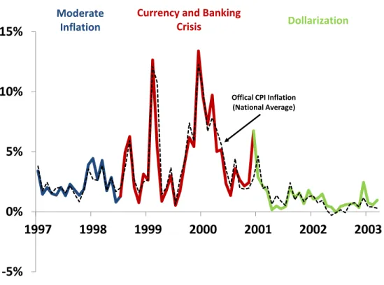
Figure 2.1 plots our monthly inflation measure together with INEC’s official Consumer Price Index. Our measure is an equally weighted average of inflation across all goods and cities. Comparing the two lines, it is obvious that our simple construct tracks the official CPI almost exactly. The inflation rate time series is shown in three colors to distinguish each inflation regime: blue for Regime 1 (Moderate regime), red for Regime 2 (the period of financial and exchange rate crisis known as the Crisis regime), and green for Regime 3 (the Dollarization regime).
Figure 2.1: Monthly CPI Inflation in Ecuador by Regime
-5%
0%
5%
10%
15%
1997 1998 1999 2000 2001 2002 2003
Moderate Inflation
Currency and Banking
Crisis Dollarization
Offical CPI Inflation (National Average)
Note: Monthly inflation rate over the sample period of January 1998 to April 2003, calculated as an equally weighted average of inflation across all goods and cities from our dataset. The black line represents the official CPI from INEC, Ecuador’s national statistical agency.
Table 2.1 presents our summary statistics across the three inflation regimes. The first row conveys the narrative history of inflation in Ecuador. In the first regime, inflation is very high compared with industrial countries, averaging 2.2 percent per month. In the second regime, during the financial and exchange rate crisis, inflation reaches hyperinflationary levels. The average is a bit deceptive in the sense that some inflationary spikes extended to more than 10 percent per month. The inflationary situation moderated in the third regime, with inflation stabilizing to 1.1 percent per month, presumably as a consequence of the dollarization together with a commitment to open trade and integration with international capital markets.
Table 2.1: Summary of Monthly Price Facts
Full sample Regime 1 Regime 2 Regime 3 Moderate regime Crisis regime Dollarization regime 1997:01-2003:04 1997:01-1998:07 1998:08-2000:12 2001:01-2003:04
Mean inflation 2.8% 2.2% 4.7% 1.1%
Price adjustment frequency 57.6% 53.9% 67.3% 50.0%
Price increases 43.2% 42.7% 54.3% 32.1%
Price declines 14.4% 11.3% 13.0% 17.9%
Size of price changes 9.1% 7.8% 11.1% 7.4%
Note: Mean inflation and price adjustment frequency are statistics across goods, cities, and time periods.The size of price changes are average absolute values across goods, cities, and time periods.
2.2.3 Price Changes in Ecuador
We now turn to individual prices and present new stylized facts observed in our novel data set. To help answer our question about the states upon which price adjustment depend, we begin with an analysis of the frequencies of price changes in Ecuador. Looking at Table 2.1, we see higher inflation periods are also periods with more frequent price changes consistent with a state-dependent or menu cost theory of price adjustment. We see this pattern consistently across the three regimes of our sample with the average frequency of price changes increasing from 50 percent (Regime 3) to 53.9 percent (Regime 1) and then to 67.3 percent (Regime 2) as we move from the lowest- to highest-inflation regime. These frequencies are about twice as high as those reported in Nakamura and Steinsson (2008) for the United States. In addition, this strong correlation between frequency of price change and inflation runs counter to much of the empirical literature (e.g., Klenow and Kryvtsov (2008)). Both of these differences are accounted for by the fact that inflation is much higher in Ecuador than in the United States, even during the most stable period of Dollarization. A more appropriate comparison of inflation rates is Gagnon (2009), who studies the frequency
of price changes in Mexico from 1994 to 2002 and shows that inflation is strongly positively correlated with price change frequency when inflation is over 10 percent (per annum). Even during the stable Dollarization regime, Ecuadorian annual inflation is about 14 percent annually. Table 2.1 also shows that higher inflation periods are associated with larger price changes as pointed out by Ahlin and Shintani (2007).
As other authors have pointed out, the frequency of price adjustment differs much more substantially across items in the consumption basket than across inflation regimes. This heterogeneity of frequencies across goods is a universal feature of micro-price data. An important question to ask is whether the cross-sectional variance in the frequency of price changes reflects an economic structure that macroeconomists should be building into their models or just uninteresting noise. We suspect that economic structure underlies these patterns.
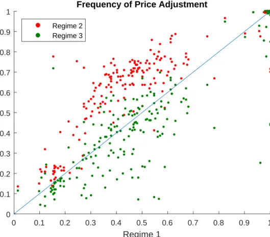
Answering a simple question has direct bearing on this issue: Does the frequency of price adjustment maintain its cross-sectional distribution as macroeconomic conditions move from one regime to another? Figure 2.2 plots the frequency of price adjustment by goods in our microsample as individual data points. The x-coordinates of this figure are the frequencies of price adjustment in Regime 1, the sample with the inflation rate closest to the historical mean. The y-coordinates for the red and green dots are the frequencies of price adjustment in Regime 2 (the Crisis regime) and Regime 3 (the Dollarization regime), re- spectively. The higher (lower) average price adjustment frequencies in Regime 2 (Regime 3) are evident with the red (green) scatter lying systematically above (below) the 45-degree line. Here we see a striking pattern in the data: items with above (or below) average fre- quencies of price adjustment in one regime are also items with above (or below) average frequencies of price adjustment in the next regime. What changes across regimes is the av- erage frequency of price change, but this is trivial relative to the dispersion in frequencies of price change across goods. This pattern is inconsistent with menu cost models in which the heterogeneity in price adjustments comes from firms drawing randomly from a com-
mon distribution of menu costs (e.g., Dotsey et al. (1999) and the open-economy versions of Landry (2009) and Landry (2010)) or from a common distribution of productivity shocks (e.g., Golosov and Lucas (2007)). In these cases, we would expect a cloud of points tightly clustered around the mean frequency in each regime with little or no pattern in relation to the 45-degree line.
Figure 2.2: Monthly Frequency of Price Adjustment in the Data
0 0.1 0.2 0.3 0.4 0.5 0.6 0.7 0.8 0.9 1
Regime 1 0
0.1 0.2 0.3 0.4 0.5 0.6 0.7 0.8 0.9
1 Frequency of Price Adjustment
Regime 2 Regime 3
Note: Comparison of price adjustment frequencies across regimes. Each dot represents one good’s frequency of price adjustment across two regimes. The x-coordinates represent the price adjustment frequencies in Regime 1, while the y-coordinates represent the price adjustment frequencies in the Regime 2 (the Crisis regime) and Regime 3 (the Dollarization regime).
Evidence of a structural relationship comes from the fact that the cross-sectional distri- bution of price adjustment frequencies is preserved across regimes. That is, the frequencies of price changes across goods is strongly positively correlated across regimes (i.e., the green and red scatter diagrams show strong positive correlation with each other). What this suggests is that there is some factor specific to an individual good that induces more- or
less-frequent price adjustments whereas the inflation regime shifts the mean frequency of price change across goods. Next, we turn to our explanation for this stable cross-sectional distribution of price adjustment frequencies.
2.3 The Model
In this section, we develop a menu cost model of pricing in which retail firms inter- mediate trade between producers and consumers. The model we develop is a multi-sector generalization of the model presented by Golosov and Lucas (2007) akin to Nakamura and Steinsson (2010)’s multisector model, but where the intermediate inputs are tradable inputs. In contrast to Nakamura and Steinsson (2010), however, we let heterogeneity in the firms’ cost structure dictate the frequency of price adjustment—instead of relying on heterogeneous menu costs.
Like traditional menu cost models, firms must pay a common fixed menu cost in order to adjust their price. However, unlike these models, each firm’s cost function may have a different weight on local and imported factors of production and, therefore leave the firm differentially exposed to the two cost shocks. Naturally, then, firms with a higher cost share of more volatile input price will adjust their prices more frequently. In most macroeconomic settings, the more volatile input prices in retail goods is the traded input component. Food and energy provide good examples due to their ties to volatile commodity prices via traded inputs. We turn now to the structural details of the model.
2.3.1 A Menu Cost Model of Price Adjustment
We develop a partial equilibrium model in which a continuum of firms indexed byibe- longs to a sector that combines labor (i.e., retail services) and a wholesale good purchased in global markets to produce a differentiated final consumption good. The production func- tion for firmiat timet is
yit =litαim1−αit i, (2.1) where yit is the final good the consumer purchases, lit denotes retail services involved in making the good available to the final consumer andmit is the intermediate-imported good.
Consumers have CES preferences over goods and thus the demand for the good i at timet is
yit=y Pit
Pt
−θ
, (2.2)
wherePit is the nominal price of goodiand the price index,Pt, is consistent with the CES preference function; it will be proxied with the CPI price index in the data. Real aggregate demand (and income) isy, andθ is the elasticity of demand.
Firmimaximizes the value of its expected discounted profits
Et
∞ s=t
∑
βt,sπis, (2.3)
whereβt,sis the discount factor between periodtand future periods. Real profits in period tare given by
πit= Pit
Ptyit−Wt
Pt lit−Pitm
Pt mit−χIit, (2.4)
whereWt is the nominal wage,Pitmis the nominal price of the intermediate imported good, Iit is an indicator variable equal to one if the firm changes its price in period t and zero otherwise, and χ is the common menu cost of price adjustment in units of aggregate con- sumption.
The price adjustment decision of a firm in our model has two dimensions: First, the price adjustment decision is a function of three relative prices: the firm’s price relative to the aggregate price level, the real wage and the real price of the intermediate-imported
good. Second, the size of the inaction region and the magnitude of the price jumps are different for each component of marginal cost, and depend on the cost share of labor and traded inputs into production. To see this more clearly, consider a log-linearized version of the nominal cost function implied by the model,
cit =αiwt+ (1−αi)pmit. (2.5) The two state variables are the wage rate in Ecuador,wt, and the import price, pmit. In our setting, the variance of the marginal cost function depends on the variance of wages, the variance of import prices, and their covariance. It also depends on the cost share of the two inputs,αi. In Golosov and Lucas (2007), the frequency of price changes is increasing in the variance of idioynscratic firm-level productivity shocks because this translates directly into higher variance in marginal cost. In our setting, however, the frequency of price adjustment depends on the cost share of the two inputs and on the variance of the wage relative to the import price. The variance of cost, assuming a zero covariance between the traded input and the wage, is
σc,i2 =αi2σw2+ (1−αi)2σim2. (2.6) Under the plausible restriction that the variance of traded input prices exceed that of wages, retail items with more traded content should reprice more frequently. However, the good or service with the lowest repricing frequency is not generally a pure labor service since a mix of inputs provides diversification against idiosyncratic factor price risk. Put differently, the U-shaped relationship between the distribution share and the total cost variance will also generally produce a U-shaped frequency of price change when plotted against the distribution share.
2.3.2 Model’s Solution and Calibration
Due to the lack of monthly wage and import price data available for Ecuador, we make two simplifying assumptions. First, we assume that the price of haircuts can be used as a proxy for the wage.3 After setting the nominal wage,Wt, equal to the price of haircuts, we rely on the model, our observed retail price, Pit, and measures of the distribution cost share from the U.S. Personal Consumption Expenditure Bridge Table to back out the import price,Pitm. Assuming constant markups and using our log-linear nominal cost function,
pit =αiwt+ (1−αi)pmit, (2.7) rearranging the equation gives the (log) price of the traded intermediate goodi
pmit = pit−αiwt
(1−αi) . (2.8)
The variablespt,wt, andpmit, form the basis of our three-variable stochastic state space:
pt =µ+pt−1+εp,t, (2.9)
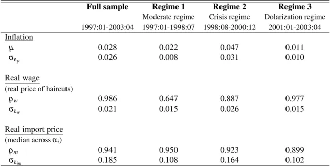
wt−pt=ρw(wt−pt) +εw,t, (2.10) pmit −pt =ρim(pmit−1−pt−1) +εim,t. (2.11) In these equation, the error terms are assumed to be normally distributed with mean zero and variancesσε2,σε2w, andσε2im. Table 2.2 gives the results of this estimation exercise.
In our benchmark calibration, we assume that all firms face the same import-price shocks (using the median volatility across regimes and goods) as this allows us to iso- late the role of heterogeneous distribution margins in accounting for the cross-sectional
3We ran an AR(1) on all non-traded goods prices for whichα>0.85 (e.g., haircuts, automobile tune-up, dry cleaning service, taxi, rent of a house). Haircut prices happens to be the AR(1) process with the median volatility among retail items with high distribution shares. Using the least volatile AR(1) process across regimes as a proxy for the wage does not change the qualitative results.
heterogeneity in price-change frequencies.4 Later in the text, we relax this assumption and look at the model’s predictions of our model when import-price shocks are heterogeneous across regimes and goods.
Table 2.2: Stochastic Properties of Shocks
Full sample Regime 1 Regime 2 Regime 3 Moderate regime Crisis regime Dolarization regime 1997:01-2003:04 1997:01-1998:07 1998:08-2000:12 2001:01-2003:04 Inflation
µ 0.028 0.022 0.047 0.011
σεp 0.026 0.008 0.031 0.010
Real wage
(real price of haircuts)
ρw 0.986 0.647 0.887 0.977
σεw 0.021 0.015 0.026 0.015
Real import price (median acrossαi)
ρm 0.941 0.950 0.923 0.899
σεim 0.185 0.108 0.164 0.102
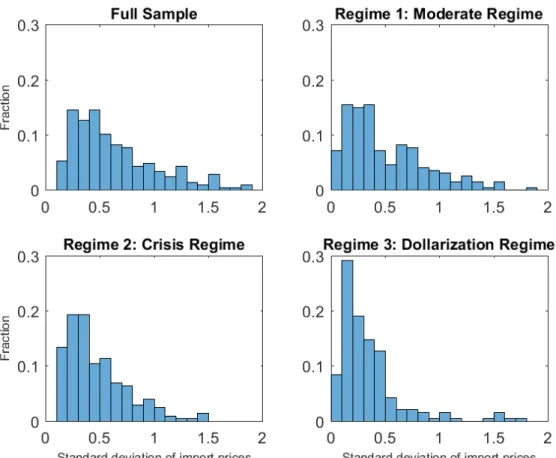
Anticipating this, Figure 2.3 is a histogram showing the variance of the import price series for each of the regimes and the full sample. As expected, the import price shocks are more widely distributed in Regime 2 and in the full sample. The heterogeneity in the veracity of import price shocks across retail items adds an additional source of heterogene- ity in price change frequency and (as we shall see) further advances the model’s ability to account for the diversity of pricing behavior exhibited in the Ecuadorian micro-data.
Firm i’s optimization problem may be written recursively in the form of the Bellman equation
4The volatility of our AR(1) processes is defined asσε2
im/(1−ρim2).
Figure 2.3: Distribution of Import Price Volatility
Note: Distribution of import prices standard deviation across regimes bins width of 0.1.
V
Pit−1 Pt ,Wt
Pt,Ptm Pt
= max {Pit}
πit+βEtV Pit
Pt+1,Wt+1 Pt+1,Pt+1m
Pt+1
, (2.12)
whereV(·) is firm i’s value function. We solve the model numerically for each firm i’s (defined by a non-traded share,αi) by iterating the Bellman operator that yields the value (2.12), and policy function on a discrete grid.
To match Ecuador’s historical data, we allow for the stochastic process of the relative prices, the real wage, and the real import price to vary across regimes according to Table 2.2. The non-traded sharesαiand the menu costχ do not change over time. We choose the menu cost so as to match the average frequency of price adjustments across firms in the full sample (i.e., 57.7 percent). This approach results in a menu cost parameter, χ, of 0.0004,
which implies that the cost of price adjustment equals about 0.60 percent of the average firm’s revenues in the full sample. Appendix B provides a full explanation of the solution method.
2.4 Results
Having estimated the stochastic processes for the two components of the firm’s cost function, we are in a position to compare our benchmark model’s predictions for the fre- quencies of price change across sectors and regimes with the micro-data. To isolate the impact of heterogeneous distribution margins, we first present results where the variance of import price shocks are the same for all firms. Then, we look into the prediction of a more realistic model in which each firm faces import price shocks with a different veracity.
2.4.1 Benchmark model
Before turning to the simulation results, it is instructive to compare the policy functions of three representative firms with different distribution shares to gain some intuition for the relationship between menu costs and price adjustment. Figure 2.4 shows the firms’ policy functions using the full sample calibration. In this figure, we hold constant the aggregate price level, the import price, and the wage.5 This is a common figure within the menu cost literature, which shows the price adjustment cutoffs as the firm’s real price fluctuates around its optimal price. In Figure 2.4, each firms has a different policy function because each firm has a different cost structure.
The sensitivity of the cost structure to cost shocks also leads firms to have slightly dif- ferent bands of inaction (or price adjustment cutoffs) relative to their optimal price. Con- sistent with our theory, we observe that firms that rely more heavily on one cost (i.e. wage
5Note that these policy functions have normalized around the firms’ optimal price, as the cost structure shifts firms’ marginal cost and optimal price.
or import prices) have wider inaction bands.6 For example, a firm that heavily rely on im- ports (e.g.,α =0.167) requires a larger deviation in its relative price to induce an optimal price change than does a firm that relies mostly on labor (e.g., α =0.931). In practice, the volatility of inputs prices is so much larger than wages that the direct effect of higher cost volatility dominates the indirect effect of the option value of waiting (widening of the bands of inaction) and prices change more frequently for retail items with more traded factor content.
Figure 2.4: Costs Variance and Policy Functions
0 0.1 0.2 0.3 0.4 0.5 0.6 0.7 0.8 0.9 1
0 1
2 Costs variance by firms, across distribution share
0.9 0.92 0.94 0.96 0.98 1 1.02 1.04 1.06 1.08 1.1
0.9 1
1.1 Policy function across three firms
=0.167
=0.751
=0.931
Note: The top panel shows the firms’ costs variance, by distribution share. The bottom panel shows the policy function of three firms with different distribution share, normalized around their optimal price in the full sample calibration, holding constant the aggregate price level, the import price, and the wage. This figure shows that firms that experience higher costs variance have larger inaction bands.
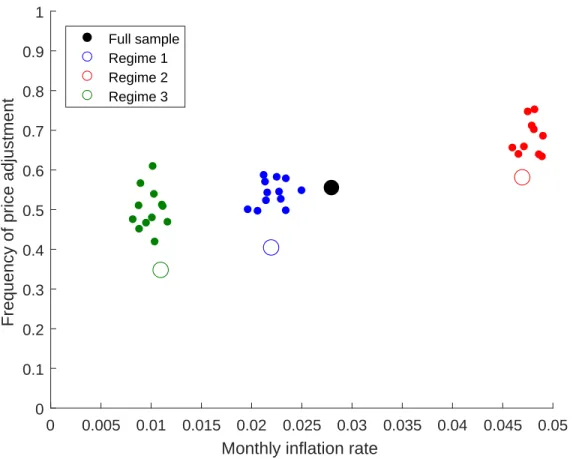
In our first exercise, we test the ability of our model to match the median frequency of prices changes across all three regimes. Figure 2.5 presents the median frequencies of price adjustments by regime for each city in the Ecuadorian micro-panel as well as the predictions of the baseline calibration of the model. The large circles are the predictions
6As pointed out by the referees, Barro (1972), and more recently Vavra (2014), increase in the volatility of input prices have two effects: First, there is a direct effect where greater volatility pushes more firms to adjust for a given region of inaction. Second, greater volatility also increases the option value of waiting, which widens the size of the inaction region and decreases the frequency of price adjustment. The first effect typically dominates with an increase in volatility, leading more frequent price adjustments despite wider inaction bands.
from the model while the small dots are the median frequency of price adjustment across cities. For example, the cluster of green dots represents the median frequencies of price adjustments across goods, city-by-city, for the Dollarization regime (Regime 3). Figure 2.5 confirms that our benchmark calibration model captures well the frequency of price adjustment across regimes.
Figure 2.5: Average Frequency of Price Adjustment by Regime, Data versus Model
0 0.005 0.01 0.015 0.02 0.025 0.03 0.035 0.04 0.045 0.05 Monthly inflation rate
0 0.1 0.2 0.3 0.4 0.5 0.6 0.7 0.8 0.9 1
Frequency of price adjustment
Full sample Regime 1 Regime 2 Regime 3
Note: Comparison of the frequency of price adjustment by regime, in the data and in the model.
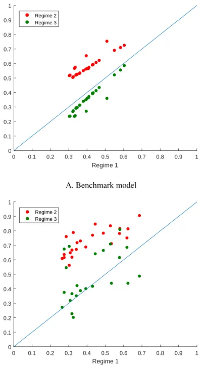
Our next exercise is to see how the model fares in accounting for the heterogeneity of price adjustment frequencies across goods. Panel A of Figure 2.7 displays the frequency of price adjustment for each distribution share in the benchmark model. In this panel, each dot represents a distribution share across the regimes in the same fashion as the data were presented in Figure 2.2: Regime 1’s simulations are on the x-axis and Regime 2’s and 3’s are the y-coordinates. It should be kept in mind that we have fewer distribution shares than
goods, which limits to some extent the cross-sectional variance that results. That being said, the variation is smaller than what we saw in Figure 2.2 earlier. We suspect that this is partly due to our adherence to a common variance of import-price shocks across goods. In the next subsection, we relax this assumption and extend the model to include heterogeneity in import prices.
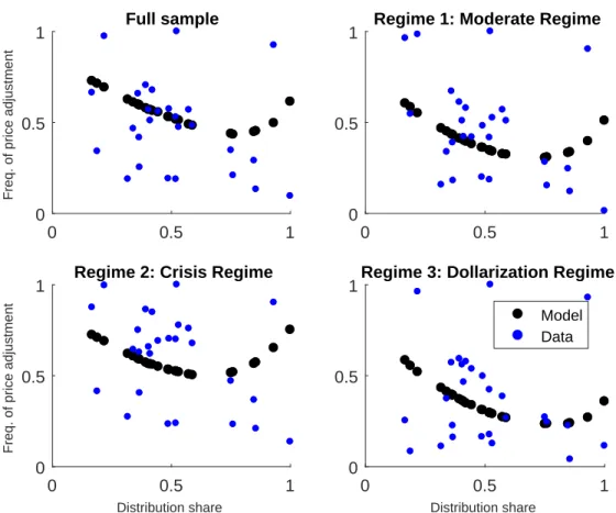
Finally, Figure 2.6 displays the relationship between the distribution share (on the x- axis) and the frequency of price adjustment (on the y-axis) in the model and in the data. The blue dots show the median frequency of price adjustment for each distribution share in the data. These dots show that firms that rely more heavily of both inputs (i.e., a distribution share close to 0.5) usually reprice less frequently than firms that rely more heavily on one input. In the model, this corresponds to the U-shape relationship discussed above and readily apparent by the black dots. Our model not only accounts for the fact that goods maintain a certain frequency of price adjustment pattern across regimes, but it also distinguishes which goods are more likely to reprice based on their cost structure.
Together, these results indicate that our menu cost model can account for many of the stylized facts we found in Section 2 and Section 3 regarding the price adjustment process of firms that are heterogeneous in their cost structure. In addition to matching the positive correlation between frequencies of price changes and aggregate inflation, our structural model provides a novel explanation for the different frequencies of price changes observed across the distribution of goods in the CPI.
2.4.1.1 Model with idiosyncratic import prices
In the baseline calibration, we use the stochastic property of the import price with the median volatility as a proxy for import prices. In this section, we extend the model to take into account differences in the volatility of import prices across retail goods. That is, we will use the stochastic property of the import price (as found in equation (2.11)) for each αifirm. We use the median volatility import-price series for each sector that has more than
Figure 2.6: Frequencies of price adjustment by regime and distribution share
0 0.5 1
0 0.5 1
Freq. of price adjustment
Full sample
0 0.5 1
0 0.5
1 Regime 1: Moderate Regime
0 0.5 1
Distribution share
0 0.5 1
Freq. of price adjustment
Regime 2: Crisis Regime
0 0.5 1
Distribution share
0 0.5
1Regime 3: Dollarization Regime Model Data
Note: The blue dots represent the median frequency of price adjustment across distribution shares in the data. The black dots represent the monthly frequency of price adjustment across firms in the model. The x-coordinate is the distribution share of the firms and the y-coordinate is the monthly frequency of price adjustment.
one retail good.7
Figure 2.7, Panel B, displays the frequency of price adjustment for each distribution share in our model with idiosyncratic import prices. As for Panel A, each dot represents a distribution share across the regimes in the same fashion as the data were presented in Figure 2.2: Regime 1’s simulations are on the x-axis and Regime 2’s and 3’s are the y- coordinates. As opposed to Panel A, however, the variation in the frequency of price ad- justment is much closer to that in Figure 2.2. In particular, the scatter plot for Regime 2 is
7In addition, Gopinath and Itskhoki (2010) and Berger and Vavra (2017) show that variation in markup elasticity across firms can generate significant variation in the frequency of price adjustment. As an alternative to our benchmark model, Appendix C looks into the pricing dynamics of firms facing variable markups.
concentrated above the 45 degree line, while that of Regime 3 are mostly below the scatter of Regime 2.
In particular, this panel speaks to Boivin et al. (2009) evidence that disaggregated prices appear sticky in response to macroeconomic and monetary disturbances but flexible in re- sponse to sector-specific shocks: Panel B shows that sector-specific shocks (i.e., idiosyn- cratic import prices) increase the frequency of price adjustment compared to the benchmark model’s where firms face common shocks (Panel A). In other words, the model with id- iosyncratic import prices generates responses to sector-level and aggregate shocks that are closer to what we observe in the data.
2.5 Conclusion
In making decisions about changes in the federal funds rate, it is essential that mon- etary policymakers distinguish generalized inflationary impulses from changes in relative prices that may affect some, but not all, market prices. The structure of our model helps to elucidate these differences. Changes in the prices of imported goods are often large and induce frequent changes in the retail prices of these goods. Essentially, this is why food and energy are typically excluded in measures of core inflation. The typical explanation for the volatility of these prices is that the markets for them are subject to particularly large sector- specific shocks. Our approach generalizes this conventional wisdom by recognizing that final goods have distinct production functions in the sense of requiring different intensities of retail labor in making them available to final consumers. This allows us to parse the in- flationary impulse of, say, an indexed wage (typically the cost-push dimension of monetary policy) from shocks that are idiosyncratic to the good or sector (such as imported goods).
Ecuador provides an ideal setting to explore this mechanism by virtue of high-frequency micro-price data by good and city spanning a varied inflationary experience.
Figure 2.7: Monthly Frequency of Price Adjustment in the Model
0 0.1 0.2 0.3 0.4 0.5 0.6 0.7 0.8 0.9 1
Regime 1 0
0.1 0.2 0.3 0.4 0.5 0.6 0.7 0.8 0.9 1
Regime 2 Regime 3
A. Benchmark model
0 0.1 0.2 0.3 0.4 0.5 0.6 0.7 0.8 0.9 1
Regime 1 0
0.1 0.2 0.3 0.4 0.5 0.6 0.7 0.8 0.9 1
Regime 2 Regime 3
B. Model with idiosyncratic import prices
Note: Comparison of price adjustment frequencies across regimes in the model. Each dot represents one firm’s frequency of price adjustment across two regimes. The x-coordinates represent the price adjustment frequencies in Regime 1, while the y-coordinates represent the price adjustment frequencies in the Regime 2 (the Crisis regime) and Regime 3 (the Dollarization regime).
Our hope is that our work will motivate similar studies in other countries to validate the menu cost model developed here using a broader cross-section of nations and inflationary environments closer to that of the United States.
Appendix A
Distribution Shares
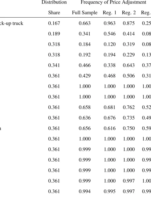
The distribution share for each good and service available in the Ecuadorian monthly database of retail prices is listed in the table below.
Table A.1 List of Goods and Services
Distribution Frequency of Price Adjustment
Item Share Full Sample Reg. 1 Reg. 2 Reg. 3
Automobile or pick-up truck 0.167 0.663 0.963 0.875 0.253
Gasoline 0.189 0.341 0.546 0.414 0.083
Newspaper 0.318 0.184 0.120 0.319 0.086
Magazine 0.318 0.192 0.194 0.229 0.136
Toilet Paper 0.341 0.466 0.338 0.643 0.374
Milk, fresh 0.361 0.429 0.468 0.506 0.318
Cheese 0.361 1.000 1.000 1.000 1.000
Eggs 0.361 1.000 1.000 1.000 1.000
Oil, vegetable 0.361 0.658 0.681 0.762 0.528
Margarine 0.361 0.636 0.676 0.735 0.497
Fruit cocktail, can 0.361 0.656 0.616 0.750 0.593
Raisins 0.361 1.000 1.000 1.000 1.000
Peas, dry 0.361 0.999 1.000 1.000 0.997
Beans, dry 0.361 0.999 1.000 1.000 0.997
Lentils 0.361 0.999 1.000 1.000 0.997
Peanuts 0.361 0.999 1.000 0.997 1.000
Sugar 0.361 0.994 0.995 0.997 0.991
Chocolate, candy 0.361 0.612 0.500 0.637 0.670
Candy 0.361 0.630 0.546 0.741 0.583
Gelatine 0.361 0.563 0.551 0.646 0.472
Marmalade 0.361 0.670 0.532 0.810 0.602
Honey 0.361 0.482 0.338 0.545 0.528
Panela 0.361 0.996 0.991 1.000 0.994
Salt 0.361 0.622 0.653 0.670 0.553
Ketchup 0.361 0.606 0.630 0.732 0.460
Broad beans, flour 0.361 0.993 1.000 1.000 0.982
Soup, dry 0.361 0.642 0.546 0.789 0.546
Coffee, ground 0.361 0.687 1.000 0.714 0.444
Coffee, instant 0.361 0.590 0.491 0.720 0.519
Cocoa 0.361 0.689 0.611 0.765 0.661
Mineral water 0.361 0.410 0.333 0.500 0.358
Soft drink, store 0.361 0.364 0.375 0.506 0.213
Orange juice 0.361 0.508 0.454 0.637 0.420
Soft drink in powder 0.361 0.381 0.389 0.449 0.303
Beer, at store 0.361 0.340 0.306 0.506 0.188
Rum 0.361 0.590 0.482 0.708 0.565
Wine 0.361 0.582 0.380 0.744 0.559
Milk of magnesia 0.361 0.453 0.509 0.637 0.232
Chicken, rotisserie 0.361 1.000 1.000 1.000 1.000
Glass 0.366 0.490 0.357 0.688 0.380
Medicines in general 0.366 0.941 0.977 0.997 0.855
Aspirin (medicine) 0.366 0.344 0.357 0.545 0.130
Linconcin (medicine) 0.366 0.472 0.458 0.696 0.219
Flagil (medicine) 0.366 0.364 0.347 0.554 0.188
Garamicina (medicine) 0.366 0.417 0.500 0.533 0.235
Neurobion (medicine) 0.366 0.414 0.245 0.753 0.179
Voltaren (medicine) 0.366 0.429 0.588 0.524 0.232
Megacilina (medicine) 0.366 0.410 0.403 0.649 0.170
Apronax (medicine) 0.366 0.428 0.463 0.643 0.179
Redoxon (medicine) 0.366 0.400 0.273 0.720 0.127
Hepabionta (medicine) 0.366 0.330 0.301 0.569 0.093
Baycuten, cream (medicine) 0.366 0.442 0.431 0.571 0.293
Comtrex (medicine) 0.366 0.422 0.426 0.634 0.201
Mucosolvan (medicine) 0.366 0.478 0.375 0.676 0.349
Cataflam (medicine) 0.366 0.460 0.528 0.619 0.262
Fungirex (medicine) 0.366 0.417 0.310 0.646 0.250
Imodium (medicine) 0.366 0.298 0.282 0.521 0.077
Acrosin-B (medicine) 0.366 0.417 0.319 0.622 0.287
Glasses 0.366 0.416 0.407 0.560 0.278
Cigarrettes 0.367 0.253 0.181 0.405 0.161
Stove, gas 0.393 0.753 0.755 0.875 0.636
Blender 0.393 0.707 0.616 0.878 0.593
Refrigerator 0.393 0.704 0.611 0.863 0.614
Pot, cooking 0.393 0.534 0.505 0.699 0.404
Cup with dish 0.393 0.472 0.417 0.661 0.318
Bleach, for laundry 0.405 0.572 0.458 0.711 0.509
Detergent 0.405 0.550 0.583 0.646 0.429
Soap for dishwashing 0.405 0.620 0.574 0.708 0.556
Soap for laundry 0.405 0.523 0.579 0.604 0.395
Cologne 0.405 0.466 0.343 0.580 0.438
Cream, moisturizer 0.405 0.598 0.500 0.679 0.580
Deodorant 0.405 0.552 0.435 0.616 0.565
Soap, deodorant 0.405 0.567 0.468 0.637 0.568
Toothpaste 0.405 0.620 0.602 0.702 0.549
Shampoo 0.405 0.537 0.361 0.625 0.574
Talc powder 0.405 0.610 0.546 0.670 0.593
Sanitary pads 0.405 0.612 0.519 0.711 0.583
TV set, color 0.411 0.721 0.611 0.848 0.673
Rent of VHS movie 0.411 0.299 0.232 0.390 0.256
Sewing machine 0.421 0.632 0.588 0.777 0.519
Iron, electric 0.421 0.640 0.537 0.857 0.494
Sound system, stereo 0.421 0.723 0.630 0.887 0.636
VCR 0.421 0.714 0.569 0.839 0.698
Shoe polish 0.445 0.571 0.389 0.696 0.583
Disinfectant, domestic 0.445 0.548 0.449 0.685 0.491
Cupboard, wooden 0.487 0.614 0.556 0.765 0.515
Bed, wooden 0.487 0.579 0.472 0.744 0.491
Chest of drawers, wooden 0.487 0.546 0.426 0.682 0.485
Matches 0.487 0.307 0.278 0.467 0.145
Book, primary school (typical) 0.487 0.141 0.144 0.164 0.127
Notebook for primary school 0.487 0.179 0.157 0.226 0.157
Notebook for secundary school 0.487 0.192 0.181 0.235 0.170
Paper, bond 0.487 0.182 0.162 0.232 0.157
Algebra book 0.487 0.190 0.218 0.202 0.173
Dictionary for school 0.487 0.130 0.148 0.140 0.117
Razor, standard manual 0.491 0.573 0.482 0.702 0.497
Cassimere, fabric 0.519 0.557 0.495 0.744 0.414
Chalis, fabric 0.519 0.566 0.389 0.765 0.488
Silk, fabric 0.519 0.433 0.315 0.607 0.340
Dress for woman, making 0.519 0.434 0.273 0.530 0.454
Pants for man, making 0.519 0.483 0.380 0.655 0.386
Suit for man, making 0.519 0.582 0.486 0.717 0.525
Socks, mens 0.519 0.507 0.431 0.711 0.367
Underwear, mens 0.519 0.561 0.477 0.735 0.454
Shirt, mens 0.519 0.550 0.560 0.711 0.380
T-shirt, mens 0.519 0.546 0.472 0.717 0.417
Pants, mens 0.519 0.623 0.574 0.768 0.528
Shorts, for sports, mens 0.519 0.512 0.380 0.679 0.441
Suit for men 0.519 0.541 0.468 0.705 0.426
T-shirt, childrens 0.519 0.590 0.500 0.708 0.531
Pants, boys 0.519 0.537 0.394 0.732 0.429
Blouse, womens, typical 0.519 0.512 0.370 0.688 0.423
Underwear, womens 0.519 0.513 0.417 0.679 0.411
T-shirt, womens 0.519 0.513 0.449 0.685 0.383
Skirt, womens 0.519 0.461 0.310 0.577 0.441
Pantyhose, nylon 0.519 0.407 0.431 0.488 0.309
Pants, womens 0.519 0.618 0.560 0.777 0.497
Dress, womens 0.519 0.501 0.380 0.667 0.420
Pants, girls 0.519 0.518 0.403 0.699 0.404
Underwear, girls 0.519 0.580 0.528 0.741 0.463
Dress, girls 0.519 0.547 0.352 0.726 0.503
Shirt, babies 0.519 0.472 0.380 0.601 0.414
Suit for baby 0.519 0.492 0.361 0.691 0.380
Shoes, leather, mens 0.519 0.558 0.463 0.759 0.414
Shoes, sneakers, mens 0.519 0.441 0.370 0.637 0.287
Shoes, boys 0.519 0.549 0.468 0.717 0.441
Shoes, leather, womens 0.519 0.568 0.472 0.753 0.451
Shoes, sneakers, womens 0.519 0.561 0.482 0.735 0.448
Shoes, girls 0.519 0.586 0.454 0.750 0.506
Shoe polishing 0.519 0.184 0.157 0.238 0.151
Dining set 0.519 0.588 0.519 0.756 0.469
Living room set 0.519 0.586 0.528 0.717 0.506
Blanket, thick, very warm 0.519 0.480 0.463 0.682 0.296
Blanket, thick, warm 0.519 0.443 0.333 0.634 0.327
Mattress 0.519 0.529 0.403 0.711 0.432
Blanket, thin 0.519 0.579 0.514 0.744 0.466
Towel 0.519 0.557 0.463 0.702 0.485
Broom 0.519 0.529 0.407 0.679 0.469
Uniform for school 0.519 0.158 0.181 0.173 0.139
School supplies in general 0.519 0.267 0.269 0.286 0.265
Compass, drawing, primary school 0.519 0.184 0.171 0.226 0.164
Ruler, primary school 0.519 0.188 0.185 0.214 0.176
Pen for primary school 0.519 0.163 0.153 0.211 0.133
Folder 0.519 0.159 0.153 0.196 0.136
Geometry set for school 0.519 0.179 0.120 0.208 0.201
Ruler, secondary school 0.519 0.184 0.194 0.214 0.161
Pen for secundary school 0.519 0.160 0.157 0.211 0.120
Diapers, disposable for children 0.519 0.542 0.435 0.640 0.522
Vegetable fat 0.523 0.591 0.597 0.685 0.469
Avocado 0.523 0.981 0.935 0.997 0.997
Bananas 0.523 0.993 0.991 0.997 0.991
Lemons 0.523 0.946 1.000 1.000 0.849
Apples 0.523 1.000 1.000 1.000 1.000
Raspberries 0.523 1.000 1.000 1.000 1.000
Oranges 0.523 0.903 0.986 1.000 0.778
Naranjilla 0.523 1.000 1.000 1.000 1.000
Papaya 0.523 1.000 1.000 1.000 1.000
Pineapple 0.523 0.998 0.991 1.000 1.000
Plantain 0.523 0.999 1.000 0.997 1.000
Watermelon 0.523 0.987 1.000 1.000 1.000
Tomatillo 0.523 1.000 1.000 1.000 1.000
Grapes 0.523 0.999 0.995 1.000 1.000
Peas, fresh 0.523 1.000 1.000 1.000 1.000
Onion, white 0.523 1.000 1.000 1.000 1.000
Onion, red 0.523 1.000 1.000 1.000 1.000
Cabbage 0.523 1.000 1.000 1.000 1.000
Cauliflower 0.523 1.000 1.000 1.000 1.000
Corn, fresh 0.523 1.000 1.000 1.000 1.000
Broad beans, fresh 0.523 1.000 1.000 1.000 1.000
Beans, fresh 0.523 1.000 1.000 1.000 1.000
Lettuce 0.523 1.000 1.000 1.000 1.000
Bell pepper 0.523 1.000 1.000 1.000 1.000
Tomatoes 0.523 1.000 1.000 1.000 1.000
Potatoes 0.523 1.000 1.000 1.000 1.000
Yucca 0.523 1.000 1.000 1.000 1.000
Carrots 0.523 1.000 1.000 1.000 1.000
Garlic 0.523 1.000 1.000 1.000 1.000
Bicycle, typical 0.531 0.473 0.565 0.801 0.074
Typewriter 0.531 0.474 0.486 0.753 0.179