Lo and Mueller (2010) Physics Envy

(1)

WARNING: Physics Envy May Be Hazardous To Your Wealth! ∗

Andrew W. Lo

^†

and Mark T. Mueller

^‡

This Draft: March 19, 2010

Abstract

The quantitative aspirations of economists and financial analysts have for many years been based on the belief that it should be possible to build models of economic systems—and financial markets in particular—that are as predictive as those in physics. While this perspective has led to a number of important breakthroughs in economics, “physics envy” has also created a false sense of mathematical precision in some cases. We speculate on the origins of physics envy, and then describe an alternate perspective of economic behavior based on a new taxonomy of uncertainty. We illustrate the relevance of this taxonomy with two concrete examples: the classical harmonic oscillator with some new twists that make physics look more like economics, and a quantitative equity market-neutral strategy. We conclude by offering a new interpretation of tail events, proposing an “uncertainty checklist” with which our taxonomy can be implemented, and considering the role that quants played in the current financial crisis.

Keywords: Quantitative Finance; Efficient Markets; Financial Crisis; History of Economic Thought.

JEL Classification: G01, G12, B16, C00

∗The views and opinions expressed in this article are those of the authors only, and do not necessarily represent the views and opinions of AlphaSimplex Group, MIT, or any of their affiliates and employees. The authors make no representations or warranty, either expressed or implied, as to the accuracy or completeness of the information contained in this article, nor are they recommending that this article serve as the basis for any investment decision—this article is for information purposes only. Research support from AlphaSimplex Group and the MIT Laboratory for Financial Engineering is gratefully acknowledged. We thank Jerry Chafkin, Peter Diamond, Arnout Eikeboom, Doyne Farmer, Gifford Fong, Jacob Goldfield, Tom Imbo, Jakub Jurek, Amir Khandani, Bob Lockner, Paul Mende, Robert Merton, Jun Pan, Roger Stein, Tina Vandersteel for helpful comments and discussion.

†Harris & Harris Group Professor, MIT Sloan School of Management, and Chief Investment Strategist, AlphaSimplex Group, LLC. Please direct all correspondence to: MIT Sloan School, 50 Memorial Drive, E52–454, Cambridge, MA 02142–1347,alo@mit.edu(email).

‡Senior Lecturer, MIT Sloan School of Management, and Visiting Scientist, MIT Department of Physics, Center for Theoretical Physics, 77 Massachusetts Avenue, Cambridge, MA 02142–1347, mark.t.mueller@mac.com(email).

(2)

1 Introduction

The Financial Crisis of 2007–2009 has re-invigorated the longstanding debate regarding the effectiveness of quantitative methods in economics and finance. Are markets and investors driven primarily by fear and greed that cannot be modeled, or is there a method to the market’s madness that can be understood through mathematical means? Those who rail against the quants and blame them for the crisis believe that market behavior cannot be quantified and financial decisions are best left to individuals with experience and discretion.

Those who defend quants insist that markets are efficient and the actions of arbitrageurs impose certain mathematical relationships among prices that can be modeled, measured, and managed. Is finance a science or an art?

In this paper, we attempt to reconcile the two sides of this debate by taking a somewhat circuitous path through the sociology of economics and finance to trace the intellectual origins of this conflict—which we refer to as “physics envy”—and show by way of example that “the fault lies not in our models but in ourselves”. By reflecting on the similarities and differences between economic phenomena and those of other scientific disciplines such as psychology and physics, we conclude that economic logic goes awry when we forget that human behavior is not nearly as stable and predictable as physical phenomena. However, this observation does not invalidate economic logic altogether, as some have argued.

In particular, if, like other scientific endeavors, economics is an attempt to understand, predict, and control the unknown through quantitative analysis, the kind of uncertainty af- fecting economic interactions is critical in determining its successes and failures. Motivated by Knight’s (1921) distinction between “risk” (randomness that can be fully captured by probability and statistics) and “uncertainty” (all other types of randomness), we propose a slightly finer taxonomy—fully reducible, partially reducible, and irreducible uncertainty—

that can explain some of the key differences between finance and physics. Fully reducible uncertainty is the kind of randomness that can be reduced to pure risk given sufficient data, computing power, and other resources. Partially reducible uncertainty contains a component that can never be quantified, and irreducible uncertainty is the Knightian limit of unparametrizable randomness. While these definitions may seem like minor extensions of Knight’s clear-cut dichotomy, they underscore the fact that there is a continuum of randomness in between risk and uncertainty, and this nether region is the domain of economics

(5)

and business practice. In fact, our taxonomy is reflected in the totality of human intellectual pursuits, which can be classified along a continuous spectrum according to the type of uncertainty involved, with religion at one extreme (irreducible uncertainty), economics and psychology in the middle (partially reducible uncertainty) and mathematics and physics at the other extreme (certainty).

However, our more modest and practical goal is to provide a framework for investors, portfolio managers, regulators, and policymakers in which the efficacy and limitations of economics and finance can be more readily understood. In fact, we hope to show through a series of examples drawn from both physics and finance that the failure of quantitative models in economics is almost always the result of a mismatch between the type of uncertainty in effect and the methods used to manage it. Moreover, the process of scientific discovery may be viewed as the means by which we transition from one level of uncertainty to the next.

This framework can also be used to extrapolate the future of finance, the subject of this special volume of the Journal of Investment Management. We propose that this future will inevitably involve refinements of the taxonomy of uncertainty and the development of more sophisticated methods for “full-spectrum” risk management.

We begin in Section 2 by examining the intellectual milieu that established physics as the exemplar for economists, inevitably leading to the “mathematization” of economics and finance. The contrast and conflicts between physics and finance can be explained by considering the kinds of uncertainty they address, and we describe this taxonomy in Section 3. We show how this taxonomy can be applied in two contexts in Sections 4 and 5, one drawn from physics (the harmonic oscillator) and the other drawn from finance (a quantitative trading strategy). These examples suggest a new interpretation of so-called “black swan” events, which we describe in Section 6. They also raise a number of practical issues that we address in Section 7, including the introduction of an “uncertainty checklist” with which our taxonomy can be applied. Finally, in Section 8 we turn to the role of quants in the current financial crisis, and consider three populist views that are either misinformed or based on incorrect claims, illustrating the benefits of a scientific approach to analysis crises.

We conclude in Section 9 with some speculation regarding the finance of the future.

Before turning to these issues, we wish to specify the intended audience for this unortho- dox and reflective article. While we hope the novel perspective we propose and the illustrative examples we construct will hold some interest for our academic colleagues, this paper can hardly be classified as original research. Instead, it is the engineer, research scientist, newly minted Wall Street quant, beleaguered investor, frustrated regulators and policymakers, and anyone else who cannot understand how quantitative models could have failed so spectac- ularly over the last few years that we intend to reach. Our focus is not on the origins of

(6)

the current financial crisis—there are now many popular and erudite accounts—but rather on developing a logical framework for understanding the role of quantitative models in theory and practice. We acknowledge at the outset that this goal is ambitious, and beg the reader’s indulgence as we attempt to reach our target audience through stylized examples and simplistic caricatures, rather than through formal theorem-and-proof.

2 Physics Envy

The fact that economics is still dominated by a single paradigm is a testament to the extraordinary achievements of one individual: Paul A. Samuelson. In 1947, Samuelson pub- lished his Ph.D. thesis titled Foundations of Economics Analysis, which might have seemed presumptuous—especially coming from a Ph.D. candidate—were it not for the fact that it did, indeed, become the foundations of modern economic analysis. In contrast to much of the extant economic literature of the time, which was often based on relatively infor- mal discourse and diagrammatic exposition, Samuelson developed a formal mathematical framework for economic analysis that could be applied to a number of seemingly unrelated contexts. Samuelson’s (1947, p. 3) opening paragraph made his intention explicit (italics are Samuelson’s):

The existence of analogies between central features of various theories implies the existence of a general theory which underlies the particular theories and unifies them with respect to those central features. This fundamental principle of generalization by abstraction was enunciated by the eminent American mathematician E.H. Moore more than thirty years ago. It is the purpose of the pages that follow to work out its implications for theoretical and applied economics.

He then proceeded to build the infrastructure of what is now known as microeconomics, routinely taught as the first graduate-level course in every Ph.D. program in economics today. Along the way, Samuelson also made major contributions to welfare economics, general equilibrium theory, comparative static analysis, and business-cycle theory, all in a single doctoral dissertation!

If there is a theme to Samuelson’s thesis, it is the systematic application of scientific principles to economic analysis, much like the approach of modern physics. This was no coincidence. In Samuelson’s (1998, p. 1376) fascinating account of the intellectual origins of his dissertation, he acknowledged the following:

Perhaps most relevant of all for the genesis of Foundations, Edwin Bidwell Wil- son (1879–1964) was at Harvard. Wilson was the great Willard Gibbs’s last (and, essentially only) prot´eg´e at Yale. He was a mathematician, a mathematical physicist, a mathematical statistician, a mathematical economist, a polymath

(7)

who had done first-class work in many fields of the natural and social sciences.

I was perhaps his only disciple . . . I was vaccinated early to understand that economics and physics could share the same formal mathematical theorems (Eu- ler’s theorem on homogeneous functions, Weierstrass’s theorems on constrained maxima, Jacobi determinant identities underlying Le Chatelier reactions, etc.), while still not resting on the same empirical foundations and certainties.

Also, in a footnote to his statement of the general principle of comparative static analysis, Samuelson (1947, p. 21) added, “It may be pointed out that this is essentially the method of thermodynamics, which can be regarded as a purely deductive science based upon certain postulates (notably the First and Second Laws of Thermodynamics)”. And much of the economics and finance literature sinceFoundations has followed Samuelson’s lead in attempting to deduce implications from certain postulates such as utility maximization, the absence of arbitrage, or the equalization of supply and demand. In fact, one of the most recent mile- stones in economics—rational expectations—is founded on a single postulate, around which a large and still-growing literature has developed.

2.1 The Mathematization of Economics and Finance

Of course, the mathematization of economics and finance was not due to Samuelson alone, but was advanced by several other intellectual giants that created a renaissance of mathematical economics during the half century following the Second World War. One of these giants, Gerard Debreu, provides an eye-witness account of this remarkably fertile period:

“Before the contemporary period of the past five decades, theoretical physics had been an inaccessible ideal toward which economic theory sometimes strove. During that period, this striving became a powerful stimulus in the mathematization of economic theory” (Debreu, 1991, p. 2).

What Debreu is referring to is a series of breakthroughs that not only greatly expanded our understanding of economic theory, but also held out the tantalizing possibility of practical applications involving fiscal and monetary policy, financial stability, and central planning.

These breakthroughs included:

• Game theory (von Neumann and Morganstern, 1944; Nash, 1951)

• General equilibrium theory (Debreu, 1959)

• Economics of uncertainty (Arrow, 1964)

• Long-term economic growth (Solow, 1956)

• Portfolio theory and capital-asset pricing (Markowitz, 1954; Sharpe, 1964; Tobin, 1958)

• Option-pricing theory (Black and Scholes, 1973; Merton, 1973)

(8)

• Macroeconometric models (Tinbergen, 1956; Klein, 1970)

• Computable general equilibrium models (Scarf, 1973)

• Rational expectations (Muth, 1961; Lucas, 1972)

Many of these contributions have been recognized by Nobel prizes, and they have permanently changed the field of economics from a branch of moral philosophy pursued by gen- tlemen scholars to a full-fledged scientific endeavor not unlike the deductive process with which Isaac Newton explained the motion of the planets from three simple laws. Moreover, the emergence of econometrics, and the over-riding importance of theory in guiding empirical analysis in economics is similar to the tight relationship between experimental and theoretical physics.

The parallels between physics and finance are even closer, due to the fact that the Black- Scholes/Merton option-pricing formula is also the solution to the heat equation. This is no accident, as Lo and Merton (2009) explain:

The origins of modern financial economics can be traced to Louis Bachelier’s magnificent dissertation, completed at the Sorbonne in 1900, on the theory of speculation. This work marks the twin births of the continuous-time mathematics of stochastic processes and the continuous-time economics of option pricing. In analyzing the problem of option pricing, Bachelier provides two different derivations of the Fourier partial differential equation as the equation for the probability density of what is now known as a Wiener process/Brownian motion. In one of the derivations, he writes down what is now commonly called the Chapman-Kolmogorov convolution probability integral, which is surely among the earlier appearances of that integral in print. In the other derivation, he takes the limit of a discrete-time binomial process to derive the continuous-time transition probabilities. Along the way, Bachelier also developed essentially the method of images (reflection) to solve for the probability function of a diffusion process with an absorbing barrier. This all took place five years before Einstein’s discovery of these same equations in his famous mathematical theory of Brownian motion.

Not surprisingly, Samuelson was also instrumental in the birth of modern financial economics (see Samuelson, 2009), and—together with his Nobel-prize-winning protege Robert C. Merton—created much of what is now known as “financial engineering”, as well as the analytical foundations of at least three multi-trillion-dollar industries (exchange-traded options markets, over-the-counter derivatives and structured products, and credit derivatives).

The mathematization of neoclassical economics is now largely complete, with dynamic stochastic general equilibrium models, rational expectations, and sophisticated economet- ric techniques having replaced the less rigorous arguments of the previous generation of economists. Moreover, the recent emergence of “econophysics” (Mantegna and Stanley,

(9)

2000)—a discipline that, curiously, has been defined not so much by its focus but more by the techniques (scaling arguments, power laws, and statistical mechanics) and occupations (physicists) of its practitioners—has only pushed the mathematization of economics and finance to new extremes.¹

2.2 Samuelson’s Caveat

Even as Samuelson wrote his remarkable Foundations, he was well aware of the limitations of a purely deductive approach. In his introduction, he offered the following admonition (Samuelson, 1947, p. 3):

. . . [O]nly the smallest fraction of economic writings, theoretical and applied, has been concerned with the derivation ofoperationally meaningful theorems. In part at least this has been the result of the bad methodological preconceptions that economic laws deduced from a priori assumptions possessed rigor and validity independently of any empirical human behavior. But only a very few economists have gone so far as this. The majority would have been glad to enunciate meaningful theorems if any had occurred to them. In fact, the literature abounds with false generalization.

We do not have to dig deep to find examples. Literally hundreds of learned papers have been written on the subject of utility. Take a little bad psychology, add a dash of bad philosophy and ethics, and liberal quantities of bad logic, and any economist can prove that the demand curve for a commodity is negatively inclined.

This surprisingly wise and prescient passage is as germane today as it was over fifty years ago when it was first written, and all the more remarkable that it was penned by a twentysome- thing year-old graduate student. The combination of analytical rigor and practical relevance was to become a hallmark of Samuelson’s research throughout his career, and despite his theoretical bent, his command of industry practices and market dynamics was astonishing.

Less gifted economists might have been able to employ similar mathematical tools and parrot his scientific perspective, but few would be able to match Samuelson’s ability to distill the economic essence of a problem and then solve it as elegantly and completely.

Unlike physics, in which pure mathematical logic can often yield useful insights and intuition about physical phenomena, Samuelson’s caveat reminds us that a purely deductive approach may not always be appropriate for economic analysis. As impressive as the achievements of modern physics are, physical systems are inherently simpler and more stable than

1However, this field is changing rapidly as physicists with significant practical experience in financial markets push the boundaries of theoretical and empirical finance; see Bouchaud, Farmer, and Lillo (2009) for an example of this new and exciting trend.

(10)

economic systems, hence deduction based on a few fundamental postulates is likely to be more successful in the former case than in the latter. Conservation laws, symmetry, and the isotropic nature of space are powerful ideas in physics that simply do not have exact counterparts in economics because of the nature of economic interactions and the types of uncertainty involved.

And yet economics is often the envy of the other social sciences, in which there are apparently even fewer unifying principles and operationally meaningful theorems. Despite the well-known factions within economics, there is significant consensus among practicing economists surrounding the common framework of supply and demand, the principle of comparative advantage, the Law of One Price, income and substitution effects, net present value relations and the time value of money, externalities and the role of government, etc.

While false generalizations certainly abound among academics of all persuasions, economics does contain many true generalizations as well, and these successes highlight important commonalities between economics and the other sciences.

Samuelson’s genius was to be able to deduce operationally meaningful theorems despite the greater uncertainty of economic phenomena. In this respect, perhaps the differences between physics and economics are not fundamental, but are due, instead, to the types of uncertainty inherent in the two respective disciplines. We expand on this possibility in Sections 3–5. Before turning to that framework, it is instructive to perform a side-by-side comparison of economics and its closest intellectual sibling—psychology.

2.3 Economics vs. Psychology

The degree of physics envy among economists is more obvious when we compare economics with the closely related field of psychology. Both disciplines focus on human behavior, so one would expect them to have developed along very similar ideological and methodological trajectories. Instead, they have developed radically different cultures, approaching human behavior in vastly different ways. Consider, first, some of the defining characteristics of psychology:

• Psychology is based primarily on observation and experimentation.

• Field experiments are common.

• Empirical analysis leads to new theories.

• There are multiple theories of behavior.

• Mutual consistency among theories is not critical.

Contrast these with the comparable characteristics of economics:

(11)

• Economics is based primarily on theory and abstraction.

• Field experiments are not common.

• Theories lead to empirical analysis.

• There are few theories of behavior.

• Mutual consistency is highly prized.

Although there are, of course, exceptions to these generalizations, they do capture much of the spirit of the two disciplines.² For example, while psychologists certainly do propose abstract theories of human behavior from time to time, the vast majority of academic psychologists conduct experiments. Although experimental economics has made important inroads into the mainstream of economics and finance, the top journals still publish only a small fraction of experimental papers, the majority of publications consisting of more tra- ditional theoretical and empirical studies. Despite the fact that new theories of economic behavior have been proposed from time to time, most graduate programs in economics and finance teach only one such theory: expected utility theory and rational expectations, and its corresponding extensions, e.g., portfolio optimization, the Capital Asset Pricing Model, and dynamic stochastic general equilibrium models. And it is only recently that departures from this theory are not dismissed out of hand; less than a decade ago, manuscripts containing models of financial markets with arbitrage opportunities were routinely rejected from the top economics and finance journals, in some cases without even being sent out to referees for review.

But thanks to the burgeoning literature in behavioral economics and finance, the Nobel prizes to Daniel Kahneman and Vernon Smith in 2002, advances in the cognitive neurosciences, and the recent financial crisis, psychological evidence is now taken more seriously by economists and finance practitioners. For example, going well beyond Keynes’ (1936)

“animal spirits”, recent research in the cognitive neurosciences has identified an important link between rationality in decision-making and emotion,³ implying that the two are not antithetical, but in fact complementary. In particular, emotions are the basis for a reward- and-punishment system that facilitates the selection of advantageous behavior, providing a numeraire for animals to engage in a “cost-benefit analysis” of the various actions open to them (Rolls, 1999, Chapter 10.3). Even fear and greed—the two most common culprits in the downfall of rational thinking, according to most behavioralists—are the product of

2For example, there is a vast econometrics literature in which empirical investigations are conducted, but almost always motivated by theory and involving an hypothesis test of one sort or another. For a less impressionistic and more detailed comparison of psychology and economics, See Rabin (1998, 2002).

3See, for example, Grossberg and Gutowski (1987), Damasio (1994), Elster (1998), Lo (1999), Lo and Repin (2002), Loewenstein (2000), and Peters and Slovic (2000).

(12)

evolutionary forces, adaptive traits that increase the probability of survival. From an evolutionary perspective, emotion is a powerful tool for improving the efficiency with which animals learn from their environment and their past. When an individual’s ability to experience emotion is eliminated, an important feedback loop is severed and his decision-making process is impaired.

These new findings imply that individual preferences and behavior may not be stable through time, but are likely to be shaped by a number of factors, both internal and external to the individual, i.e., factors related to the individual’s personality, and factors related to specific environmental conditions in which the individual is currently situated. When environmental conditions shift, we should expect behavior to change in response, both through learning and, over time, through changes in preferences via the forces of natural selection.

These evolutionary underpinnings are more than simple speculation in the context of financial market participants. The extraordinary degree of competitiveness of global financial markets and the outsize rewards that accrue to the “fittest” traders suggest that Darwinian selection is at work in determining the typical profile of the successful investor. After all, un- successful market participants are eventually eliminated from the population after suffering a certain level of losses.

This perspective suggests an alternative to the antiseptic world of rational expectations and efficient markets, one in which market forces and preferences interact to yield a much more dynamic economy driven by competition, natural selection, and the diversity of individual and institutional behavior. This approach to financial markets, which we refer to as the “Adaptive Markets Hypothesis” (Farmer and Lo, 1999; Farmer, 2002; Lo, 2004, 2005;

and Brennan and Lo, 2009), is a far cry from theoretical physics, and calls for a more sophisticated view of the role that uncertainty plays in quantitative models of economics and finance. We propose such a view in Section 3.

3 A Taxonomy of Uncertainty

The distinctions between the various types of uncertainty are, in fact, central to the differences between economics and physics. Economists have been aware of some of these distinctions for decades, beginning with the University of Chicago economist Frank Knight’s (1921) Ph.D. dissertation in which he distinguished between two types of randomness: one that is amenable to formal statistical analysis, which Knight called “risk”, and another that is not, which he called “uncertainty”. An example of the former is the odds of winning at the roulette table, and an example of the latter is the likelihood of peace in the Middle East

(13)

within the next five years. Although Knight’s motivation for making such a distinction is different from ours—he was attempting to explain why some businesses yield little profits (they take on risks, which easily become commoditized) while others generate extraordinary returns (they take on uncertainty)—nevertheless, it is a useful starting point for understanding why physics seems so much more successful than economics. In this section, we propose an even more refined taxonomy of uncertainty, one capable of explaining the differences across the entire spectrum of intellectual pursuits from physics to biology to economics to philosophy and religion.

3.1 Level 1: Complete Certainty

This is the realm of classical physics, an idealized deterministic world governed by Newton’s laws of motion. All past and future states of the system are determined exactly if initial conditions are fixed and known—nothing is uncertain. Of course, even within physics, this perfectly predictable clockwork universe of Newton, Lagrange, LaPlace, and Hamilton was recognized to have limited validity as quantum mechanics emerged in the early twentieth century. Even within classical physics, the realization that small perturbations in initial conditions can lead to large changes in the subsequent evolution of a dynamical system underscores how idealized and limited this level of description can be in the elusive search for truth.

However, it must be acknowledged that much of the observable physical universe does, in fact, lie in this realm of certainty. Newton’s three laws explain a breathtakingly broad span of phenomena—from an apple falling from a tree to the orbits of planets and stars—and has done so in the same manner for more than 10 billion years. In this respect, physics has enjoyed a significant head start when compared to all the other sciences.

3.2 Level 2: Risk without Uncertainty

This level of randomness is Knight’s (1921) definition of risk: randomness governed by a known probability distribution for a completely known set of outcomes. At this level, probability theory is a useful analytical framework for risk analysis. Indeed, the modern axiomatic foundations of probability theory—due to Kolmogorov, Wiener, and others—is given precisely in these terms, with a specified sample space and a specified probability measure.

No statistical inference is needed, because we know the relevant probability distributions exactly, and while we do not know the outcome of any given wager, we know all the rules and the odds, and no other information relevant to the outcome is hidden. This is life in

(14)

a hypothetical honest casino, where the rules are transparent and always followed. This situation bears little resemblance to financial markets.

3.3 Level 3: Fully Reducible Uncertainty

This is risk with a degree of uncertainty, an uncertainty due to unknown probabilities for a fully enumerated set of outcomes that we presume are still completely known. At this level, classical (frequentist) statistical inference must be added to probability theory as an appropriate tool for analysis. By “fully reducible uncertainty”, we are referring to situations in which randomness can be rendered arbitrarily close to Level-2 uncertainty with sufficiently large amounts of data using the tools of statistical analysis. Fully reducible uncertainty is very much like an honest casino, but one in which the odds are not posted and must therefore be inferred from experience. In broader terms, fully reducible uncertainty describes a world in which a single model generates all outcomes, and this model is parameterized by a finite number of unknown parameters that do not change over time and which can be estimated with an arbitrary degree of precision given enough data.

The resemblance to the “scientific method”—at least as it is taught in science classes today—is apparent at this level of uncertainty. One poses a question, develops a hypothesis, formulates a quantitative representation of the hypothesis (i.e., a model), gathers data, analyzes that data to estimate model parameters and errors, and draws a conclusion. Human interactions are often a good deal messier and more nonlinear, and we must entertain a different level of uncertainty before we encompass the domain of economics and finance.

3.4 Level 4: Partially Reducible Uncertainty

Continuing our descent into the depths of the unknown, we reach a level of uncertainty that now begins to separate the physical and social sciences, both in philosophy and model- building objectives. By Level-4 or “partially reducible” uncertainty, we are referring to situations in which there is a limit to what we can deduce about the underlying phenomena generating the data. Examples include data-generating processes that exhibit: (1) stochastic or time-varying parameters that vary too frequently to be estimated accurately; (2) nonlin- earities too complex to be captured by existing models, techniques, and datasets; (3) nonstationarities and non-ergodicities that render useless the Law of Large Numbers, Central Limit Theorem, and other methods of statistical inference and approximation; and (4) the dependence on relevant but unknown and unknowable conditioning information.

Although the laws of probability still operate at this level, there is a non-trivial degree of

(15)

uncertainty regarding the underlying structures generating the data that cannot be reduced to Level-2 uncertainty, even with an infinite amount of data. Under partially reducible uncertainty, we are in a casino that may or may not be honest, and the rules tend to change from time to time without notice. In this situation, classical statistics may not be as useful as a Bayesian perspective, in which probabilities are no longer tied to relative frequencies of repeated trials, but now represent degrees of belief. Using Bayesian methods, we have a framework and lexicon with which partial knowledge, prior information, and learning can be represented more formally.

Level-4 uncertainty involves “model uncertainty”, not only in the sense that multiple models may be consistent with observation, but also in the deeper sense that more than one model may very well be generating the data. One example is a regime-switching model in which the data are generated by one of two possible probability distributions, and the mechanism that determines which of the two is operative at a given point in time is also stochastic, e.g., a two-state Markov process as in Hamilton (1989, 1990). Of course, in principle, it is always possible to reduce model uncertainty to uncertainty surrounding the parameters of a single all-encompassing “meta-model”, as in the case of a regime-switching process. Whether or not such a reductionist program is useful depends entirely on the complexity of the meta-model and nature of the application.

At this level of uncertainty, modeling philosophies and objectives in economics and finance begin to deviate significantly from those of the physical sciences. Physicists believe in the existence of fundamental laws, either implicitly or explicitly, and this belief is often accompanied by a reductionist philosophy that seeks the fewest and simplest building blocks from which a single theory can be built. Even in physics, this is an over-simplification, as one era’s “fundamental laws” eventually reach the boundaries of their domains of validity, only to be supplanted and encompassed by the next era’s “fundamental laws”. The classic example is, of course, Newtonian mechanics becoming a special case of special relativity and quantum mechanics.

It is difficult to argue that economists should have the same faith in a fundamental and reductionist program for a description of financial markets (although such faith does persist in some, a manifestation of physics envy). Markets are tools developed by humans for accomplishing certain tasks—not immutable laws of Nature—and are therefore subject to all the vicissitudes and frailties of human behavior. While behavioral regularities do exist, and can be captured to some degree by quantitative methods, they do not exhibit the same level of certainty and predictability as physical laws. Accordingly, model-building in the social sciences should be much less informed by mathematical aesthetics, and much more by pragmatism in the face of partially reducible uncertainty. We must resign ourselves to

(16)

models with stochastic parameters or multiple regimes that may not embody universal truth, but are merely useful, i.e., they summarize some coarse-grained features of highly complex datasets.

While physicists make such compromises routinely, they rarely need to venture down to Level 4, given the predictive power of the vast majority of their models. In this respect, economics may have more in common with biology than physics. As the great mathematician and physicist John von Neumann observed, “If people do not believe that mathematics is simple, it is only because they do not realize how complicated life is”.

3.5 Level 5: Irreducible Uncertainty

Irreducible uncertainty is the polite term for a state of total ignorance; ignorance that cannot be remedied by collecting more data, using more sophisticated methods of statistical inference or more powerful computers, or thinking harder and smarter. Such uncertainty is beyond the reach of probabilistic reasoning, statistical inference, and any meaningful quantification.

This type of uncertainty is the domain of philosophers and religious leaders, who focus on not only the unknown, but the unknowable.

Stated in such stark terms, irreducible uncertainty seems more likely to be the excep- tion rather than the rule. After all, what kinds of phenomena are completely impervious to quantitative analysis, other than the deepest theological conundrums? The usefulness of this concept is precisely in its extremity. By defining a category of uncertainty that cannot be reduced to any quantifiable risk—essentially an admission of intellectual defeat—we force ourselves to stretch our imaginations to their absolute limits before relegating any phenomenon to this level.

3.6 Level ∞ : Zen Uncertainty

Attempts to understand uncertainty are mere illusions; there is only suffering.

3.7 The Uncertainty Continuum

As our sequential exposition of the five levels of uncertainty suggests, whether or not it is possible to model economic interactions quantitatively is not a black-and-white issue, but rather a continuum that depends on the nature of the interactions. In fact, a given phenomenon may contain several levels of uncertainty at once, with some components being completely certain and others irreducibly uncertain. Moreover, each component’s categorization can vary over time as technology advances or as our understanding of the phenomenon deepens.

(17)

For example, 3,000 years ago solar eclipses were mysterious omens that would have been considered Level-5 uncertainty, but today such events are well understood and can be predicted with complete certainty (Level 1). Therefore, a successful application of quantitative methods to modeling any phenomenon requires a clear understanding of the level of uncertainty involved.

In fact, we propose that the failure of quantitative models in economics and finance is almost always attributable to a mismatch between the level of uncertainty and the methods used to model it. In Sections 4–6, we provide concrete illustrations of this hypothesis.

4 The Harmonic Oscillator

To illustrate the import of the hierarchy of uncertainty proposed in Section 3, in this section we apply it to a well-known physical system: the simple harmonic oscillator. While trivial from a physicist’s perspective, and clearly meant to be an approximation to a much more complex reality, this basic model of high-school physics fits experimental data far better than even the most sophisticated models in the social sciences. Therefore, it is an ideal starting point for illustrating the differences and similarities between physics and finance.

After reviewing the basic properties of the oscillator, we will inject certain types of noise into the system and explore the implications for quantitative models of its behavior as we proceed from Level 1 (Section 4.1) to Level 4 (Section 4.4). As more noise is added, physics begins to look more like economics.⁴ We postpone a discussion of Level-5 uncertainty until Section 6, where we provide a more expansive perspective in which phenomena transition from Level 5 to Level 1 as we develop deeper understanding of their true nature.

4.1 The Oscillator at Level 1

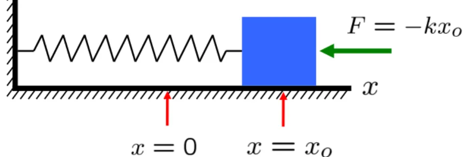
Consider a mass situated at the originx= 0 of a frictionless surface, and suppose it is attached to a spring. The standard model for capturing the behavior of this one-dimensional system when the mass is displaced from the origin—which dates back to 1660—is that the spring exerts a restoring force F which is proportional to the displacement and in the opposite direction (see Figure 1); that is, F = −kx where k is the spring constant and x is the position of the mass m. This hypothetical relation works so well in so many circumstances that physicists refer to it as a “law”, Hooke’s Law, in honor of its discoverer, Robert Hooke.

4However, we must emphasize the illustrative nature of this example, and caution readers against too literal an interpretation of our use of the harmonic oscillator with noise. We are not suggesting that such a model is empirically relevant to either physics or economics. Instead, we are merely exploiting its simplicity to highlight the differences between the two fields.

(18)

Figure 1: Frictionless one-dimensional spring system.

By applying Newton’s Second Law (F = ma) to Hooke’s Law, we obtain the following second-order linear differential equation:

¨ x + k

mx = 0 (1)

where ¨xdenotes the second time-derivative ofx. The solution to (1) is well-known and given by:

x(t) = A cos(ωot+φ) (2)

where ωo ≡ p

k/m and A and φ are constants that depend on the initial conditions of the system. This is the equation for a harmonic oscillator with amplitude A, initial phase angle φ, period T = 2πp

m/k, and frequency f = 1/T. Despite its deceptively pedestrian origins, the harmonic oscillator is ubiquitous in physics, appearing in contexts from classical mechanics to quantum mechanics to quantum field theory, and underpinning a surprisingly expansive range of theoretical and applied physical phenomena.

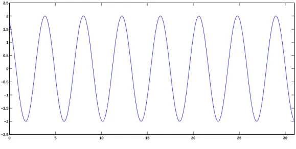
At this stage, the model of the block’s position (2) is capturing a Level-1 phenomenon, perfect certainty. For parameters A = 2, ωo = 1.5, and φ= 0.5, Figure 2 traces out the displacement of the block without error—at time t = 3.5, we know with certainty that x= 1.7224.

(19)

0 5 10 15 20 25 30

−2.5

−2

−1.5

−1

−0.5 0 0.5 1 1.5 2 2.5

Figure 2: Time series plot of the displacement x(t) =Acos(ωot+φ) of a harmonic oscillator with parameters A= 2, ωo= 1.5, and φ= 0.5.

4.2 The Oscillator at Level 2

As satisfying as this knowledge is, physicists are the first to acknowledge that (2) is an ide- alization that is unlikely to be observed with real blocks and springs. For example, surface and air friction will dampen the block’s oscillations over time, and the initial displacement cannot exceed the spring’s elastic limit otherwise the spring could break or be permanently deformed. Such departures from the idealized world of (2) will cause us to leave the com- forting world of Newtonian mechanics and Level-1 certainty.

For the sake of exposition, consider the simplest departure from (2), which is the introduction of an additive noise term to the block’s displacement:

x(t) = Acos(ωot+φ) + ǫ(t) , ǫ(t) IID N(0, σ²_ǫ) (3) where ‘IID’ stands for “independently and identically distributed”, N(0, σ_ǫ²) indicates a normal distribution with mean 0 and variance σ²_ǫ, and all parameters, including σ_ǫ², are fixed and known.⁵ Althoughx(t) is no longer deterministic, Level-2 uncertainty implies that the probabilistic structure of the displacement is completely understood. While we can no

5This example of Level-2 uncertainty corresponds to a number of actual physical phenomena, such as thermal noise in elements of an electronic circuit, where the analogue of the parameterσ²_ǫ is related in a fundamental way to the temperature of the system, described by an instance of a fluctuation-dissipation theorem, Nyquist’s theorem (Reif, 1965, Chapter 15).

(20)

longer say with certainty that at time t= 3.5, x= 1.7224, we do know that if σǫ= 0.15, the probability that x falls outside the interval [1.4284,2.0164] is precisely 5%.

4.3 The Oscillator at Level 3

Level 3 of our taxonomy of uncertainty is fully-reducible uncertainty, which we have defined as uncertainty that can be reduced arbitrarily closely to pure risk (Level 2) given a sufficient amount of data. Implicit in this definition is the assumption that the future is exactly like the past in terms of the stochastic properties of the system, i.e., stationarity.⁶ In the case of the harmonic oscillator, this assumption means that the oscillator (2) is still the data- generating process with fixed parameters, but the parameters and the noise distribution are unknown:

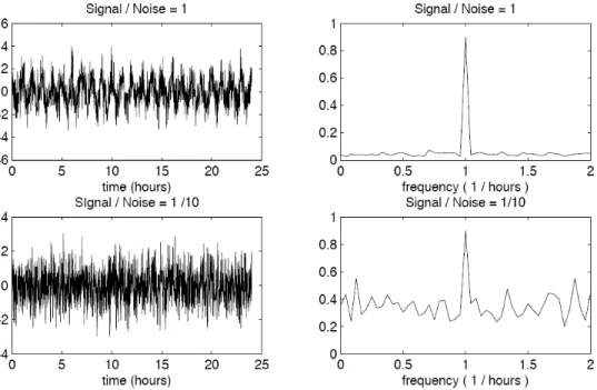
x(t) = Acos(ωot+φ) + ǫ(t) , E[ǫ(t)] = 0 , E[ǫ(t1)ǫ(t2)] = 0 ∀ t1 6=t2 . (4) However, under Level-3 uncertainty, we can estimate all the relevant parameters arbitrarily accurately with enough data, which is a trivial signal-processing exercise. In particular, although the timescale and the units in which the amplitude is measured in (4) are completely arbitrary, for concreteness let the oscillator have a period of 1 hour given a 24-hour time sample period. With data sampled every minute, this system yields a sample size of 1,440 observations.⁷ Assuming a signal-to-noise ratio of 0.1 and applying the Fast Fourier Trans- form (FFT) to this time series yields an excellent estimate of the oscillator’s frequency, as Figure 3 demonstrates. If this system were even a coarse approximation to business cycles and stock market fluctuations, economic forecasting would be a trivial task.

4.4 The Oscillator at Level 4

We now turn to Level-4 uncertainty, the taxon in which uncertainty is only partially reducible. To illustrate the characteristics of this level, suppose that the displacement x(t) is

6In physics, the stationarity of physical laws is often taken for granted. For example, fundamental relationships such as Newton’sF=mahave been valid over cosmological time scales, and appear to be accurate descriptions of many physical phenomena from very early in the history of the Universe (Weinberg, 1977).

Economics boasts no such equivalents. However, other physical systems exhibit localized nonstationarities that fall outside Level-3 uncertainty (e.g., the properties of semiconductors as they are subjected to time- varying and non-stationary temperature fluctuations, vibration, and electromagnetic radiation), and entire branches of physics are devoted to such non-stationarities, e.g., non-equilibrium statistical mechanics.

7Alternatively, for those who may wish to picture a system with a longer time scale, this example can be interpreted as sampling daily observations of the oscillator with a period of 60 days over a total time period of slightly less that four years.

(21)

Figure 3: Simulated time series and Fourier analysis of displacements xt of a harmonic oscillator with a period of 1 hour, sampled at 1-minute intervals over a 24-hour period, with signal-to-noise ratio of 1 (top graphs) and 0.10 (bottom graphs).

not governed by a single oscillator with additive noise, but is subject to regime shifts between two oscillators without noise (we will consider the case of an oscillator with additive noise below). Specifically, let:

x(t) = I(t)x1(t) + 1−I(t)

x2(t) (5a)

xi(t) = Aicos(ωit+φi) , i= 1,2 (5b) where the binary indicator I(t) determines which of the two oscillators x1(t) or x2(t) is generating the observed processx(t), and letI(t) be a simple two-state Markov process with the following simple transition probability matrix P:

P ≡

I(t) = 1 I(t) = 0 I(t−1) = 1 1−p p I(t−1) = 0 p 1−p

!

. (6)

(22)

As before, we will assume that we observe the system once per minute over a timespan of 24 hours, and let the two oscillators’ periods be 30 and 60 minutes, respectively; their dimensionless ratio is independent of the chosen timescale, and has been selected arbitrarily.

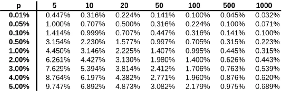
Although the most general transition matrix could allow for different probabilities of exiting each state, for simplicity we have taken these probabilities to be equal to a common valuep.

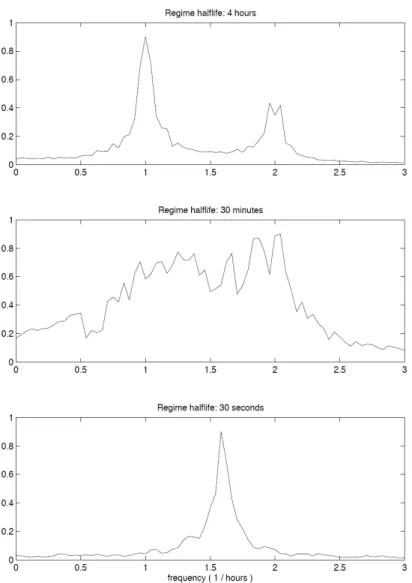
The value ofp determines the half-life of remaining in a given state, and we will explore the effects of varying p. We also impose restrictions on the parameters of the two oscillators so that the observed displacement x(t) and its first time-derivative ˙x(t) are continuous across regime switches, which ensures that the observed time series do not exhibit sample-path discontinuities or “structural breaks”.⁸ This example of Level-4 uncertainty illustrates one possible form of the stochastic behavior of the oscillator frequency, namely a regime switching model. Such stochastic oscillators can be useful in building models of a variety of physical systems (see Gitterman, 2005). For example, the description of wave propagation in random media involves the behavior of certain types of stochastic oscillators, as in the propagation of sound waves through the ocean.

In keeping with our intention to illustrate Level-4 uncertainty, suppose that none of the details of the structure of x(t) are known to the observer attempting to model this system.

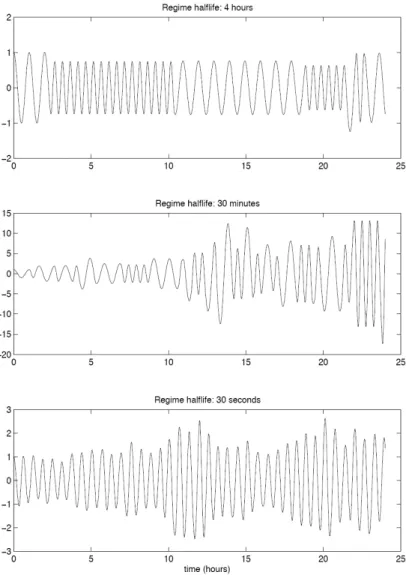
Figure 4 shows three different examples of the observed time series x(t) generated by (5).

Each panel corresponds to a different value for the switching probability p: the top panel corresponds to a half-life of 4 hours (significantly greater than the periods of either oscillator);

the middle panel corresponds to a half-life of 30 minutes (the same period as oscillator 1 and comparable to oscillator 2); and the bottom panel corresponds to a half-life of 30 seconds (considerably shorter than the period of both oscillators).

In these cases, the behavior of x(t) is less transparent than in the single-oscillator case.

However, in the two extreme cases where the values ofpimply either a much greater or much smaller period than the two oscillators, there is hope. When the regime half-life is much

8Specifically, we require that at any regime-switching time, the block’s position and velocity are continuous. Of course the block’s second time-derivative, i.e., its acceleration, will not be continuous across switching times. Therefore, in transiting from regimeiwith angular frequency ωi to regimej with angular frequencyωj, we require thatAicos(ωi∆ti+φi) =Ajcos(φj) andAiωisin(ωi∆ti+φi) =Ajωjsin(φj), where

∆ti is the time the system has just spent in regimei, which is known at the time of the transition. These equations have a unique solution forAj andφj in terms ofAi andφi:

A²_j=A²_i[cos²(ωi∆ti+φi) + (ωi/ωj)²sin²(ωi∆ti+φi)] , tan(φj) = (ωi/ωj) tan(ωi∆ti+φi) In simulatingx(t), these equations are applied iteratively, starting from the chosen initial conditions at the beginning of the sample, and the regime shifts are governed by the Markov chain (6).

It is also worth mentioning that energy is not conserved in this system, since the switching of frequencies can be characterized as some external influence injecting or extracting energy from the oscillator. Accordingly, the amplitude of the observed time series can and does change, and the system is unstable in the long run.

(23)

Figure 4: Simulated time series of a harmonic oscillator with regime-switching parameters in which the probability of a regime switch is calibrated to yield a regime half-life of 4 hours (top panel), 30 minutes (middle panel), and 30 seconds (bottom panel). The oscillator’s parameters are completely specified by the half-life (or equivalently the transition probability) and the frequencies in each regime.

(24)

greater than both oscillators’ periods, enough data can be collected during each of the two regimes to discriminate between them. In fact, visual inspection of the Fourier transform depicted in the top panel of Figure 5 confirms this intuition. At the other extreme, when the regime half-life is much shorter than the two oscillators’ periods, the system behaves as if it were a single oscillator with a frequency equal to the harmonic mean of the two oscillators’

frequencies, and with an amplitude that is stochastically modulated. The Fourier transform in the bottom panel of Figure 5 confirms that a single effective frequency is present. Despite the fact that two oscillators are, in fact, generating the data, for all intents and purposes, modeling this system as a single oscillator will yield an excellent approximation.

The most challenging case is depicted in the middle panel of Figure 5, which corresponds to a value ofpthat implies a half-life comparable to the two oscillators’ periods. Neither the time series nor its Fourier transform offers any clear indication as to what is generating the data. And recall that these results do not yet reflect the effects of any additive noise terms as in (4).

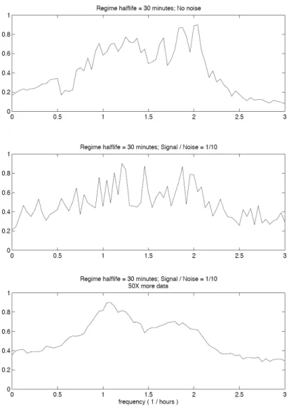
If we add Gaussian white noise to (5), the signal-extraction process becomes even more challenging, as Figure 6 illustrates. In the top panel, we reproduce the Fourier transform of the middle panel of Figure 5 (that is, with no noise), and in the two panels below, we present the Fourier transforms of the same regime-switching model with additive Gaussian noise, calibrated with the same parameters as in the middle panel of Figure 5 for the oscillators, and with the additive noise component calibrated to yield a signal-to-noise ratio of 0.1. The middle panel of Figure 6 is the Fourier transform of this new simulation using the same sample size as in Figure 5, and the bottom panel contains the Fourier transform applied to a dataset 50 times larger. There is no discernible regularity in the oscillatory behavior of the middle panel, and only when we use significantly more data do the two characteristic frequencies begin to emerge.

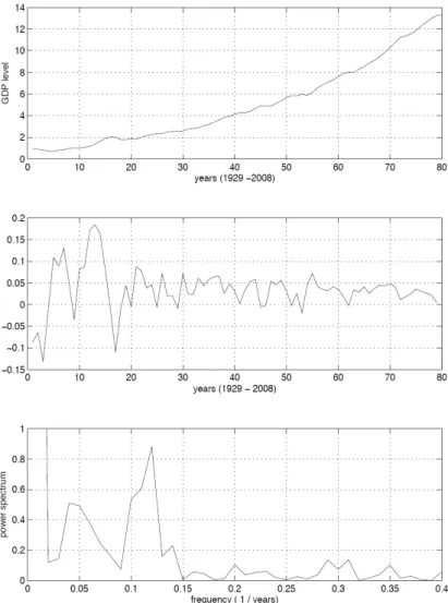
The relevance of Level-4 uncertainty for economics is obvious when we compare the middle panel of Figure 6 to the Fourier transform of a standard economic time series such as growth rates for U.S. real gross domestic product from 1929 to 2008, displayed in the bottom panel of Figure 7. The similarities are striking, which may be why Paul Samuelson often quipped that “economists have predicted five out of the past three recessions”.

Note the markedly different data requirements between this model with Level-4 uncertainty and those with Level-3 uncertainty. Considerably more data is needed just to identify the presence of distinct regimes, and this is a necessary but not sufficient condition for accurate estimation of the model’s parameters, i.e., the oscillator frequencies, the transition matrix for the Markov process, and the variance of the additive noise. Moreover, even if we are able to obtain sufficient data to accurately estimate the model’s parameters, it may still

(25)

Figure 5: Fast Fourier transforms of the simulated time series of a harmonic oscillator with regime-switching parameters in which the probability of a regime switch is calibrated to yield a regime half-life of 4 hours (top panel), 30 minutes (middle panel), and 30 seconds (bottom panel). The oscillator’s parameters are completely specified by the half-life (or equivalently the transition probability) and the frequencies in each regime.

(26)

Figure 6: Fast Fourier transforms of simulated time series the two-state regime-switching harmonic oscillator with additive noise. For comparison, the case without additive noise and where the regime half-life is comparable to the oscillators’ periods is given in the top panel. The middle panel corresponds to the case with additive noise and regime half-life comparable to the oscillators’ periods, and the bottom panel is the same analysis applied to a dataset 50 times longer than the other two panels.

(27)

Figure 7: Annual levels (top panel), growth rates (middle panel), and Fourier transform of U.S. GDP (bottom panel) in 2005 dollars, from 1929 to 2008.

(28)

be impossible to construct reliable forecasts if we cannot identify in real time which regime we currently inhabit. In the financial markets context, such a model implies that even if markets are inefficient—in the sense that securities returns are not pure random walks—we may still be unable to profit from it, a particularly irksome state of affairs that might be called the “Malicious Markets Hypothesis”.

If Tycho, Kepler, Galileo and Newton had been confronted with such “quasi-periodic”

data for the cyclical paths of the planets, it may have taken centuries, not years, of observa- tional data for them to arrive at the same level of understanding of planetary motion that we have today. Fortunately, as challenging as physics is, much of it apparently does not operate at this level of uncertainty. Unfortunately, financial markets can sometimes operate at an even deeper level of uncertainty, uncertainty that cannot be reduced to any of the preceding levels simply with additional data. We turn to this level in Section 6, but before doing so, in the next section we provide an application of our taxonomy of uncertainty to a financial context.

5 A Quantitative Trading Strategy

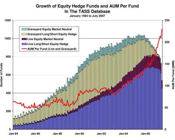
Since the primary focus of this paper is the limitations of a physical-sciences approach to financial applications, in this section we apply our taxonomy of uncertainty to the mean- reversion strategy of Lehmann (1990) and Lo and MacKinlay (1990a), in which a portfolio of stocks is constructed by buying previous under-performing stocks, and short-selling previous outperforming stocks by the same dollar amount. This quantitative equity market-neutral strategy is simple enough to yield analytically tractable expressions for its statistical properties, and realistic enough to illustrate many of the practical challenges of this particular part of the financial industry, which has come to be known as “statistical arbitrage” or “statarb”.

This strategy has been used more recently by Khandani and Lo (2007, 2008) to study the events surrounding the August 2007 “Quant Meltdown”, and the exposition in this section closely follows theirs. To parallel our sequential exposition of the oscillator in Section 4, we begin in Section 5.1 with those few aspects of statarb that may be interpreted as Level-1 certainty, and focus on progressively more uncertain aspects of the strategy in Sections 5.2–

5.4. As before, we will postpone any discussion of Level-5 uncertainty to Section 6 where we address the full range of uncertainty more directly.

(29)

5.1 StatArb at Level 1

Perhaps the most obvious difference between physics and financial economics is the fact that almost no practically relevant financial phenomena falls into the category of Level 1, perfect certainty. The very essence of finance is the interaction between uncertainty and investment decisions, hence in a world of perfect certainty, financial economics reduces to standard microeconomics. Unlike the oscillator of Section 4, there is no simple deterministic model of financial markets that serves as a useful starting point for practical considerations, except perhaps for simple default-free bond-pricing formulas and basic interest-rate calculations.

For example, consider a simple deterministic model of the price Pt of a financial security:

Pt = Pt−1 + Xt (7)

where Xt is some known increment. If Xt is known at date t−1, then a positive value will cause investors to purchase as many shares of the security as possible in anticipation of the price appreciation, and a negative value will cause investors to short-sell as many shares as possible to profit from the certain price decline. Such behavior implies that Pt will take on only one of two extreme values—0 or ∞—which is clearly unrealistic. Any information regarding future price movements will be exploited to the fullest extent possible, hence deterministic models like (7) are virtually useless in financial contexts except for the most elementary pedagogical purposes.

5.2 StatArb at Level 2

Consider a collection ofN securities and denote byRttheN×1-vector of their date-treturns [R1t· · ·RN t]^′. To be able to derive the statistical properties of any strategy based on these security returns, we require the following assumption:

(A1) Rtis a jointly covariance-stationary multivariate stochastic process with known distribution, which we take to be Gaussian with expectation and autocovariances:

E[Rt] ≡ µ = [µ1 µ2 · · · µN]^′ E[(Rt−k−µ)(Rt−µ)^′] ≡ Γk

where, with no loss of generality, we let k ≥0 since Γk =Γ^′−k.

(30)

This assumption is the embodiment of Level-2 uncertainty where the probability distributions of all the relevant variables are well-defined, well-behaved, and stable over time.⁹

Given theseN securities, consider a long/short market-neutral equity strategy consisting of an equal dollar amount of long and short positions, where at each rebalancing interval, the long positions consist of “losers” (underperforming stocks, relative to some market average) and the short positions consist of “winners” (outperforming stocks, relative to the same market average). Specifically, if ωit is the portfolio weight of security i at datet, then

ωit(k) = − 1

N(Rit−k−Rmt−k) , Rmt−k ≡ 1 N

N

X

i=1

Rit−k (8)

for some k > 0. By buying the previous losers and selling the previous winners at each date, such a strategy actively bets on mean reversion across all N stocks, profiting from reversals that occur within the rebalancing interval.¹⁰ For this reason, (8) has been called a

“contrarian” trading strategy that benefits from overreaction, i.e., when underperformance is followed by positive returns and vice-versa for outperformance. Also, since the portfolio weights are proportional to the differences between the market index and the returns, securities that deviate more positively from the market at time t−k will have greater negative weight in the date-tportfolio, and vice-versa. Also, observe that the portfolio weights are the negative of the degree of outperformancek periods ago, so each value ofk yields a somewhat different strategy. Lo and MacKinlay (1990a) provide a detailed analysis of the unleveraged returns (9) of the contrarian trading strategy, tracing its profitability to mean reversion in individual stock returns as well as positive lead/lag effects and cross-autocorrelations across stocks and across time.

Note that the weights (8) have the property that they sum to 0, hence (8) is an example of an “arbitrage” or “market-neutral” portfolio where the long positions are exactly offset by the short positions.¹¹ As a result, the portfolio “return” cannot be computed in the

9The assumption of multivariate normality in (A1) is not strictly necessary for the results in this section, but is often implicitly assumed, e.g., in Value-at-Risk computations of this portfolio’s return, in the exclusive focus on the first two moments of return distributions, and in assessing the statistical significance of associated regression diagnostics.

10However, Lo and MacKinlay (1990a) show that this need not be the only reason that contrarian investment strategies are profitable. In particular, if returns are positively cross-autocorrelated, they show that a return-reversal strategy will yield positive profits on average, even if individual security returns are serially independent. The presence of stock market overreaction, i.e., negatively autocorrelated individual returns, enhances the profitability of the return-reversal strategy, but is not required for such a strategy to earn positive expected returns.

11Such a strategy is more accurately described as a “dollar-neutral” portfolio since dollar-neutral does not necessarily imply that a strategy is also market-neutral. For example, if a portfolio is long $100MM of high-

(31)

standard way because there is no net investment. In practice, however, the return of such a strategy over any finite interval is easily calculated as the profit-and-loss of that strategy’s positions over the interval divided by the initial capital required to support those positions.

For example, suppose that a portfolio consisting of $100MM of long positions and $100MM of short positions generated profits of $2MM over a one-day interval. The return of this strategy is simply $2MM divided by the required amount of capital to support the $100MM long/short positions. Under Regulation T, the minimum amount of capital required is $100MM (often stated as 2 : 1 leverage, or a 50% margin requirement), hence the return to the strategy is 2%. If, however, the portfolio manager is a broker-dealer, then Regulation T does not apply (other regulations govern the capital adequacy of broker-dealers), and higher levels of leverage may be employed. For example, under certain conditions, it is possible to support a $100MM long/short portfolio with only $25MM of capital—leverage ratio of 8 : 1—which implies a portfolio return of $2/$25 = 8%.¹² Accordingly, the gross dollar investment Vt of the portfolio (8) and its unleveraged (Regulation T) portfolio return Rpt are given by:

Vt ≡ 1 2

N

X

i=1

|ωit| , Rpt ≡ PN

i=1ωitRit

Vt

. (9)

To construct leveraged portfolio returnsLpt(θ) using a regulatory leverage factor of θ: 1, we simply multiply (9) by θ/2:¹³

Lpt(θ) ≡ (θ/2)PN

i=1ωitRit

Vt

. (10)

Because of the linear nature of the strategy, and Assumption (A1), the strategy’s statistical properties are particularly easy to derive. For example, Lo and MacKinlay (1990a)

beta stocks and short $100MM of low-beta stocks, it will be dollar-neutral but will have positive market-beta exposure. In practice, most dollar-neutral equity portfolios are also constructed to be market-neutral, hence the two terms are used almost interchangeably.

12The technical definition of leverage—and the one used by the U.S. Federal Reserve, which is responsible for setting leverage constraints for broker-dealers—is given by the sum of the absolute values of the long and short positions divided by the capital, so:

|$100|+| −$100|

$25 = 8.

13Note that Reg-T leverage is, in fact, considered 2:1 which is exactly (9), henceθ: 1 leverage is equivalent to a multiple ofθ/2.

(32)

show that the strategy’s profit-and-loss at datet is given by:

πt(k) = ω^′<