These chapters provide the basis for the four theories covered in the last half of the book: queuing theory, game theory, control theory and information theory. The Discrete-Time-and-Frequency Fourier Transform and the Fast Fourier Transform (FFT) 157 The Fast Fourier Transform 159 .
Probability
Introduction
- Outcomes
- Events
- Disjunctions and conjunctions of events
- Axioms of probability
- Subjective and objective probability
Continuing with example 1, we define the mutually exclusive events {1,2} and {3,4} that both have a probability of 1/3. The axiomatic approach does not care how the probability of an event is determined.
Joint and conditional probability
- Joint probability
- Conditional probability
- Bayes’ rule
Let P(UDP) denote the probability that the packet is of type UDP and let P(52) denote the probability that the packet is of length 52 bytes. This allows us to calculate the probability of any one of the priors Ei, conditional on the occurrence of the posterior F.
Random variables
- Distribution
- Cumulative density function
- Generating values from an arbitrary distribution
- Expectation of a random variable
- Variance of a random variable
We can use a similar approach to generate values from a continuous random variable with the associated density function f(Xc). Intuitively, the expected value of a random variable is the value we expect it to take, knowing nothing else about it.

Moments and moment generating functions
- Moments
- Moment generating functions
- Properties of moment generating functions
Thus, the MGF represents all moments of the random variable X in a single compact expression. If the random variable X has an MGF M(t), then the MGF of the random variable Y = a+bX eatM(bt).
Standard discrete distributions
- Bernoulli distribution
- Binomial distribution
- Geometric distribution
- Poisson distribution
What is the probability that we will see at least one packet on the link during any one second interval. The probability that we see at least one packet on the link during a one-second interval is therefore:

Standard continuous distributions
- Uniform distribution
- Gaussian or Normal distribution
- Exponential distribution
- Power law distribution
The expected value of a Gaussian random variable with parameters and is and its variance is. Suppose the time taken by a teller at a bank is an exponentially distributed random variable with an expected value of one minute.

Useful theorems
- Markov’s inequality
- Chebyshev’s inequality
- Chernoff bound
- Strong law of large numbers
- Central limit theorem
Assume that the probability of success of each iteration is independent of the others (this is critical!). First, we calculate the MGF of the sum of n random variables in terms of the MGFs of each of the random variables.

Jointly distributed random variables
- Bayesian networks
This greatly reduces the amount of information required to describe the joint probability distribution of the random variables. The joint distribution of the random variables (L, A, D, T, R) will assign a probability to each possible combination of the variables, such as p (packet loss AND no ack loss AND no duplicate ack AND timeout AND no retransmission) .

Further Reading
Exercises
Assuming that outgoing calls are independent and that a guest room has 10 minutes of outgoing calls during the busiest hour of the day, what is the probability that five calls are active at the same time during the busiest hour. You are told that the time between meteors is exponentially distributed, with an average of 200 seconds.
Statistics
Sampling a population
- Types of sampling
- Scales
- Outliers
Targeted: Here, the idea is to sample only elements that meet a specific definition of the population. Convenience: A convenience sample involves studying those elements of the population that happen to be conveniently available.
Describing a sample parsimoniously
- Tables
- Bar graphs, histograms, and cumulative histograms
- The sample mean
- The sample median
- Measures of variability
The variance of the sample mean (ie, the variance of the sampling distribution of the mean) can be calculated as follows. Therefore, the variance of the sample mean is 1/n of the variance of the population variance.

Inferring population parameters from sample parameters
The variance of the sample distribution (ie of X) is σ2/n, so it has a narrower spread than the population (with the spread decreasing as we increase the number of elements in the sample). We can obtain the appropriate confidence intervals for the population variance by studying the sampling distribution of the var-.

Testing hypotheses about outcomes of experiments
- Hypothesis testing
- Errors in hypothesis testing
- Formulating a hypothesis
- Comparing an outcome with a fixed quantity
- Comparing outcomes from two experiments
- Testing hypotheses regarding quantities measured on ordinal scales
- Fitting a distribution
- Power
The power of a statistical test is the probability that the test rejects a null hypothesis when it is in fact false. Then the probability that we reject the null hypothesis (which is false) is essentially the same as the significance level (why?).
Independence and dependence: regression, and correlation
- Independence
- Regression
- Correlation
We calculate the chi-square statistic as the sum of squares of the variable (observed value - expected value)2/(expected value). It is informative to look at the scatterplot of the data, shown in Figure 5(a).

Comparing multiple outcomes simultaneously: analysis of variance
- One-way layout
- Multi-way layouts
SSB/(I-1) is also an unbiased estimator of the population variance because it is an unbiased estimator. For example, to quantify the degree of effect, we can calculate the regression of the observed effect as a function of the treatment.
Design of experiments
For example, we might want to study the joint effect of buffer size and traffic load on the loss rate. The details of this so-called two-sided representation are beyond the scope of this text.
Dealing with large data sets
Note that to perform repeated joins, we need to define the distance between a point and a cluster and between two clusters. The distance between a point and a cluster can be defined either as the distance from that point to the nearest point in the cluster or as the average of all the distances from that point to all the points in the cluster.
Common mistakes in statistical analysis
- What is the population?
- Lack of confidence intervals in comparing results
- Not stating the null hypothesis
- Too small a sample
- Too large a sample
- Not controlling all variables when collecting observations
- Converting ordinal to interval scales
- Ignoring outliers
Remember that we can only reject or not reject the null hypothesis from observational data. If the sample size is too large, a sample that deviates even slightly from the null hypothesis will cause the null hypothesis to be rejected.
Further reading
Therefore, when interpreting a test that rejects the null hypothesis, it is important to consider the effect size, which is the (subjective) degree to which the rejection of the null hypothesis accurately reflects reality. However, in the context of the problem, the value 0.005 is indistinguishable from zero, and therefore has a small 'effect'. In this case, we would still not reject the null hypothesis.
Exercises
If the number of peers were independent of uplink capacity, what is the expected value of the number of peers for a given uplink capacity?. Using the chi-square test, can we conclude that the number of peers is independent of uplink performance at the 95% and 99.9% confidence levels?.
Linear Algebra
Vectors and matrices
Unlike a vector, whose elements may not be related, elements in the same column of a matrix are usually related to each other. Existence of distinct additive and multiplicative identity elements in the set: There are distinct elements denoted by "0" and.
Vector and matrix algebra
- Addition
- Transpose
- Multiplication
- Square matrices
- Exponentiation
- Matrix exponential
The product of two vectors can be defined as either a dot product or a cross product. Therefore, the product of an n-dimensional row vector - a matrix of size - with a matrix is a row vector of dimension n.
Linear combinations, independence, basis, and dimension
- Linear combinations
- Linear independence
- Vector spaces, basis, and dimension
Note that if a set of vectors is not linearly independent, each of them can be rewritten in terms of the others (why?). What is the set of vectors that can be created as linear combinations of this set.
Solving linear equations using matrix algebra
- Representation
- Elementary row operations and Gaussian elimination
- Rank
- Determinants
- Cramer’s theorem
- The inverse of a matrix
This vector can be expressed as a linear combination of the basis set as x = ax1 + bx2 + cx3. Note that the rank of a matrix is equal to the cardinality of the basis set of the corresponding set of row vectors.
Linear transformations, eigenvalues and eigenvectors
- A matrix as a linear transformation
- The eigenvalue of a matrix
- Computing the eigenvalues of a matrix
- Why are eigenvalues important?
- The role of the principal eigenvalue
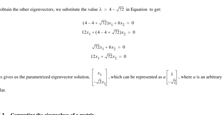
- Finding eigenvalues and eigenvectors
- Similarity and diagonalization
As we have seen, the eigenvalues of the matrix are the roots of the characteristic polynomial. Then it can be easily shown, by expanding the underlying terms, that the matrix.
Stochastic matrices
- Computing state transitions using a stochastic matrix
We have combined these results to argue that the power method can be used to calculate the stationary probability distribution of a stochastic matrix. The power technique for finding the dominant eigenvector of a stochastic matrix can be used to rank a series of web pages.

Exercises
Use the power method to calculate the dominant eigenvalue and the corresponding eigenvector of the matrix. If it is known that the initial state is state 1 with probability 0.5 and state 2 with probability 0.5, calculate the probability of being in these two states after two time steps.
Optimization
- System modelling and optimization
- An introduction to optimization
- Optimizing linear systems
- Network flow
- Integer linear programming
- Total unimodularity
- Weighted bipartite matching
- Dynamic programming
- Nonlinear constrained optimization
- Lagrangian techniques
- Karush-Kuhn-Tucker conditions for nonlinear optimization
- Heuristic non-linear optimization
- Hill climbing
- Genetic algorithms
- Exercises
The optimal value of O is reached for values of xis corresponding to the optimal peak. We want to find the set of tuples of the form (x,y) that maximize f(x,y) subject to the constraint g(x,y) = c.

Signals, Systems, and Transforms
Introduction
Background
- Sinusoids
- Complex numbers
- Euler’s formula
- Discrete-time convolution and the impulse function
- Continuous-time convolution and the Dirac delta function
Given the importance of rotating vectors (also called phasors), it is desirable to compactly display the current vector position on a unit disk. Note that each convolution value of x(t) and y(t) (ie at time t) is the result of summing all product pairs and.

Signals
- The complex exponential signal
A signal that often appears in the study of transformations is the complex exponential signal denoted , where k is a real number and s is a complex quantity that can be written as It is worth studying these numbers carefully because they provide deep insight into the nature of a complex exponential that will greatly help in understanding the nature of transformations.
Systems
- Types of systems
As discussed in Section 8.3.2 on page 226, in the context of control theory, the transfer function is more accurately described as the Laplace transform of the system's impulse response. At this stage, however, this loose but intuitively appealing description of the transfer function will suffice.
Analysis of a linear time-invariant system
- The effect of an LTI system on a complex exponential input Consider an LTI system that is described by
- The output of an LTI system with a zero input
- The output of an LTI system for an arbitrary input
- Stability of an LTI system
Therefore, the response of the system is its natural response (except at time 0 itself). Since the system is linear, the response of the system to a scaled impulse will be a scaled output, so that.
Transforms
Consider the complex exponential which represents a solution to the characteristic equation of an LTI system (Equation 23). Finally, if all the values of σ are 0, then the behavior of the system depends on whether there are repeated roots.
The Fourier series
Solution: The kth coefficient of the Fourier series corresponding to this function is given by. Note that the coefficients ck are real functions of τ (not t), which is a parameter of the input signal.

The Fourier Transform
- Properties of the Fourier transform
Calculate the Fourier transform of a single rectangular pulse of height 1 and width centered on the origin (Figure 11). Calculate the Fourier transform of a rectangular pulse as in Figure 11 but with a pulse width of.

The Laplace Transform
- Poles, Zeroes, and the Region of convergence
- Properties of the Laplace transform
This is called the pole of the system (the pole in the previous example was at 0). If the region of convergence of the Laplace transform of a signal includes an imaginary axis, then the Fourier transform of the signal is defined and can be obtained by setting.

The Discrete Fourier Transform and Fast Fourier Transform
- The impulse train
- The discrete-time Fourier transform
- Aliasing
- The Fast Fourier Transform
Due to the linearity of the Fourier transform, we can simply calculate the transform of a single value. This defines the discrete-time Fourier transform of the discrete function x[nT] and is denoted.

The Z Transform
- Relationship between Z and Laplace transform
- Properties of the Z transform
We now discuss how the z-auxiliary variable of the Z-transform relates to the s-auxiliary variable used in the Laplace transform. Note that the vertical line marked with a diamond lies in the left half-plane of the s-plane.

Further Reading
To find the inverse transform, remember that the Z-transform is linear, so we only need to find the . From Row 3 and Row 5 of Table 6 we get , which is a discrete unit step of height 2 to which is added a decaying discrete exponential.
Exercises
1 Complex arithmetic
2 Phase angle
3 Discrete convolution
4 Signals
5 Complex exponential
6 Linearity
7 LTI system
8 Natural response
9 Natural response
10 Stability
11 Fourier series
12 Fourier series
13 Fourier transform
14 Inverse Fourier transform
15 Computing the Fourier transform
16 Laplace transform
17 Laplace transform
18 Solving a system using the Laplace transform
19 Discrete-time Fourier transform
20 Discrete-time-and-frequency Fourier transform
21 Z transform
22 Z transform
Stochastic Processes and Queueing Theory
- Overview
- A general queueing system
- Little’s theorem
- Stochastic processes
- Discrete and continuous stochastic processes
- Markov processes
- Homogeneity, state transition diagrams, and the Chapman-Kolmogorov equations
- Irreducibility
- Recurrence
- Periodicity
- Ergodicity
- A fundamental theorem
- Stationary (equilibrium) probability of a Markov chain
- A second fundamental theorem
In this case, the family of random variables corresponding to the stochastic process consists of the variables X(t1), X(t2),. Therefore, the random variable corresponding to the state of the process can take real values, and the corresponding stochastic process would be a continuous space process.

In an irreducible and aperiodic homogeneous Markov chain, the limiting probability distribution
- Mean residence time in a state
- Continuous-time Markov Chains
- Markov property for continuous-time stochastic processes
- Residence time in a continuous-time Markov chain
- Stationary probability distribution for a continuous-time Markov chain
- Birth-Death processes
- Time-evolution of a birth-death process
- Stationary probability distribution of a birth-death process
- Finding the transition-rate matrix
- A pure-birth (Poisson) process
- Stationary probability distribution for a birth-death process
- The M/M/1 queue
- Two variations on the M/M/1 queue
- The M/M/ queue: a responsive server
- M/M/1/K: bounded buffers
We thus obtain the long-run probabilities of being in any state j as a function of the probability of being in state 0 and the system parameters. Note that the long-run probability that the population size j depends only on the use of the system.


