No part of this publication may be reproduced, stored in a retrieval system, or transmitted in any form or by any means, electronic, mechanical, photocopying, recording, scanning, or otherwise, except as permitted by section 107 or 108 of the United States 1976. of the State Copyright Act, without the prior written permission of the publisher or authorization by paying the appropriate copy fee to Copyright Clearance Center, Inc., 222 Rosewood Drive, Danvers, MA by fax or online at www.copyright .com. Disclaimer/Disclaimer: Although the publisher and author have used their best efforts in the preparation of this book, they make no representations or warranties as to the accuracy or completeness of the contents of this book and expressly disclaim any implied warranties of merchantability or fitness for a specific purpose.
PREFACE
ACKNOWLEDGMENTS
ABOUT THE AUTHOR
OPTICS TECHNOLOGY FOR DEFENSE SYSTEMS
OPTICAL RAYS
PARAXIAL OPTICS
In 1840, Gauss proposed the paraxial approximation for the propagation of rays that remain close to the axis of an optical system. In this case, the propagation is, say, in this direction and the light changes in transverse directions and directions only at a small distance relative to the distance that is related to the radius of curvature of the spherically curved surface and xandy (Fig. 1.1).
GEOMETRIC OR RAY OPTICS .1 Fermat’s Principle
- Fermat’s Principle Proves Snell’s Law for Refraction
- Limits of Geometric Optics or Ray Theory
- Fermat’s Principle Derives Ray Equation
- Useful Applications of the Ray Equation
- Matrix Representation for Geometric Optics
Therefore, in a numerical calculation, we discretize the refractive index profile into piecewise constant segments and obtain a piecewise linear optical ray path in plane-y. We will use in Section 2.1.2 the 2×2 notation with matrix elements labeled clockwise from the top left as ABCD to calculate the effect of propagating a Gaussian beam through the corresponding optical element.

OPTICS FOR LAUNCHING AND RECEIVING BEAMS
- Imaging with a Single Thin Lens
- Beam Expanders
- Beam Compressors
- Telescopes
- Microscopes
- Spatial Filters
A concave mirror (Figure 1.4c) performs a function similar to the convex lens by focusing parallel rays of light. From the lens law, equation (1.24), using a negative sign because it is on the opposite side of the lens compared to Figure 1.5.

GAUSSIAN BEAMS AND POLARIZATION
GAUSSIAN BEAMS
- Description of Gaussian Beams
- Gaussian Beam with ABCD Law
- Forming and Receiving Gaussian Beams with Lenses
The imaginary part of the reciprocal of the last term in equation (2.11) times λ/π defines the beam radius W(z) from. Thus, by induction, for any optical element, equation (2.20) will provide the information about the propagation of a Gaussian beam.

POLARIZATION
- Wave Plates or Phase Retarders
- Stokes Parameters
- Poincar ´e Sphere
- Finding Point on Poincar ´e Sphere and Elliptical Polarization from Stokes Parameters
- Controlling Polarization
The quarter-wave plate causes aφ=π/2 phase shift of the phase φ of the x-polarization relative to their polarization. If the polarization drifts with time, it will create a time path on the surface of the sphere.

OPTICAL DIFFRACTION
INTRODUCTION TO DIFFRACTION
- Description of Diffraction
- Review of Fourier Transforms
The magnitude of the Fourier transform of a square pulse or boxcar is shown in Figure 3.2c. The spatial Fourier transform will separate the plane waves into several discrete points in the spatial frequency domain (Section 14.1).

UNCERTAINTY PRINCIPLE FOR FOURIER TRANSFORMS
- Uncertainty Principle for Fourier Transforms in Time
- Uncertainty Principle for Fourier Transforms in Space
We show that the square root of the right-hand side of equation (3.8) leads to E/2, which is the quotient of the right-hand side of the uncertainty principle, equation (3.5);. First, the square root of the right-hand side of equation (3.8) can be written as

SCALAR DIFFRACTION
- Preliminaries: Green’s Function and Theorem
- Field at a Point due to Field on a Boundary
- Diffraction from an Aperture
- Fresnel Approximation
- Fraunhofer Approximation
- Role of Numerical Computation
To apply Green's theorem, equation (3.24), we require, at the boundary, the field U and the normal field ∂U/∂n (Figure 3.5). Now using a similar process (using a bar over a variable to represent a unit vector) as for equation (3.28), but substituting 01.

DIFFRACTION-LIMITED IMAGING
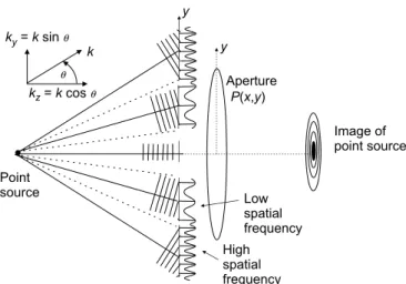
- Intuitive Effect of Aperture in Imaging System
- Computing the Diffraction Effect of a Lens Aperture on Imaging
We now show how to calculate the effect of the aperture on an output image. This requires that the impulse response from input to output be a delta function of the form (|M|2 is added to conserve total power). Equation (3.64) is the Fraunhofer diffraction of the diaphragm; note the scale byλdi in the pupil function for Fraunhofer.
DIFFRACTIVE OPTICAL ELEMENTS
- APPLICATIONS OF DOEs
- DIFFRACTION GRATINGS
- Bending Light with Diffraction Gratings and Grating Equation A beam of light can be bent by both diffraction (Figure 4.2c) and refraction (Fig-
- Cosinusoidal Grating
- Performance of Grating
- ZONE PLATE DESIGN AND SIMULATION
- Appearance and Focusing of Zone Plate
- Zone Plate Computation for Design and Simulation
- GERCHBERG–SAXTON ALGORITHM FOR DESIGN OF DOEs The Gerchberg–Saxton algorithm [43, 69, 152], is an error reduction algorithm to
- Goal of Gerchberg–Saxton Algorithm
- Inverse Problem for Diffractive Optical Elements
- Gerchberg–Saxton Algorithm for Forward Computation
A 3D view of the relief area plate is shown in Figure 4.6b and a section through it is shown in Figure 4.7. The solid line in Figure 4.10 shows the normalized output intensity at the back focal plane for the area plate illuminated with aligned coherent light. Therefore, the peak intensity for the surface relief zone plate is twice that of the blocking zone plate.

PROPAGATION AND COMPENSATION FOR ATMOSPHERIC TURBULENCE
STATISTICS INVOLVED
- Ergodicity
- Locally Homogeneous Random Field Structure Function
We now find the relation between the 1D spatial spectrum Vuin equation (5.15) and the spatial power spectrum for a 3D statistically homogeneous isotropic medium (for which radiusR= |R2−R1|). Therefore, the 3D spatial power spectrum for a locally statistically homogeneous isotropic medium, u(κ) in equation (5.17), is related to the 1D spatial power spectrum for a locally statistically homogeneous medium, Vu(κ) in equation (5.15), by . We note that some approaches to optical turbulence use the spatial power spectrum and some the structure function.
OPTICAL TURBULENCE IN THE ATMOSPHERE
- Kolmogorov’s Energy Cascade Theory
- Power Spectrum Models for Refractive Index in Optical Turbulence
- Atmospheric Temporal Statistics
- Long-Distance Turbulence Models
Power spectrum for the Kolmogorov spectrum: From Section 5.2.1, the Kolmogorov spectrum for the refractive index has the same shape as that for the velocity; therefore, replacing equation Cvin (5.24) with Cng gives Truncation of the spectrum at the large-scale limit, where the frequency is lowest, is undesirable because equation (5.32) shows that the energy in the turbulence is greatest at this limit, leading to large abrupt transitions that provide an unrealistic spectrum. Tatar spectrum and modified Von Karman spectrum: The Kolmogorov spectrum can be modified by extending it above and below the limits by the appropriate multipliers of equation (5.32).
ADAPTIVE OPTICS
- Devices and Systems for Adaptive Optics
The lower half of the wavefront is focused on the lower parts of the sensor array. In beam cleaning, the wavefront is flattened into a plane wave by placing the deformable mirror in the conjugate phase of the wavefront. For example, we can shift to the right the mirror element of the deformable mirror that aligns with the wave front in the direction along the beam at C (Figure 5.3a).

COMPUTATION OF LASER LIGHT THROUGH ATMOSPHERIC TURBULENCE
- Layered Model of Propagation Through Turbulent Atmosphere In the layered model (Figure 5.5), the propagation distance is split into layers of
- Generation of Kolmogorov Phase Screens by the Spectral Method
- Generation of Kolmogorov Phase Screens from Covariance Using Structure Functions
In this section, we generate phase screens directly from the Kolmogorov spectrum using methods described in the literature. Since the Kolmogorov model has less high spatial frequencies, the phase screens have a similar spectral smoothing. The result again agrees with the Kolmogorov spectrum shown in Figure 5.6, suggesting that the covariance matrix approach is as effective as the spectral method (Section 5.4.2) for generating phase screens.

OPTICAL INTERFEROMETERS AND OSCILLATORS
OPTICAL INTERFEROMETERS
- Michelson Interferometer
- Mach–Zehnder Interferometer
- Optical Fiber Sagnac Interferometer
If the environment changes the propagation time in one arm of the interferometer, there will be a phase difference on the screen. In the case of the subsequent fiber optic and integrated optic versions, the light is scattered into the cladding by destructive interference. Rotating the system on a rotating platform (lazy Susan) results in light traveling different distances in the two directions to reach a common photodetector chip.

FABRY–PEROT RESONATORS
- Fabry–Perot Principles and Equations
- Fabry–Perot Equations
- Piezoelectric Tuning of Fabry–Perot Tuners
We conclude that resonance only occurs when the distance across the etalonx is a multiple of half wavelengths λ/2, as shown in Figure 6.12 and by using β=2π/λ in equation (6.22). H(f)H(f)∗. FIGURE 6.14 Longitudinal frequency modes from Fabry-Perot resonator. 6.28) where τ is the single travel time to travel through the etalon. Previously, we represented modes in terms of the number of half-wavelength cycles that fit into the distance across the cavity width x (Equation (6.23) and Figure 6.12).

THIN-FILM INTERFEROMETRIC FILTERS AND DIELECTRIC MIRRORS
- Applications for Thin Films
- Forward Computation Through Thin-Film Layers with Matrix Method
- Inverse Problem of Computing Parameters for Layers
The amplitude of the reflection will also depend on the refractive indices across the interfaces, equation (6.36). In this case, an element of the Jacobian matrix can be computed. 6.54) From equation (6.54), the four product terms are partial calculations for the forward calculation. The refractive indices are now updated for the next (m+1)th iteration of the generalized inverse algorithm (Figure 6.20).

LASER TECHNOLOGY FOR DEFENSE SYSTEMS
PRINCIPLES FOR BOUND ELECTRON STATE LASERS
LASER GENERATION OF BOUND ELECTRON STATE COHERENT RADIATION
- Advantages of Coherent Light from a Laser
- Basic Light–Matter Interaction Theory for Generating Coherent Light
Some advantages of coherent light radiation are discussed in this section from the system point of view. We show that a pump and a resonator are required to create coherent light radiation in a coupled electron state laser. Equation (7.8) shows that the Einstein coefficient for the spontaneous emission rate, which gives rise to the incoherent noise, is proportional to the Einstein coefficient for the stimulated emission rate, the desired coherent light.

SEMICONDUCTOR LASER DIODES
- p–n Junction
- Semiconductor Laser Diode Gain
- Semiconductor Laser Dynamics
- Semiconductor Arrays for High Power
The lowest order mode field for the generated light shows that light is trapped in the active layer shown in Figure 7.7e. If the power gain per unit length is in the active material and α is the internal absorption per unit length, for a round trip between facets in the cavity of lengthL[176] (Figure 7.8) we can have the amplitude gain (factor 2 for two) write -away and square root of amplitude) as [eg2L]1/2=egL and the absorption as [e−α2L]1/2=e−αL. The gain of the active material in the laser diode at the nominal wavelength λ0 depends on the injected pump current density, J A/m2, and other parameters.

SEMICONDUCTOR OPTICAL AMPLIFIERS
The level in the photon density reservoir increases over time by the amount of the modified stimulated emission reductionvgg(N)Nph from the carrier density reservoir and decreases due to a photon decay time constantτph that represents the time a photon remains in the cavity (longer for highly reflective mirrors). If remnants of the resonance still appear appreciably, the SOA is known as a Fabry-Perot SOA. In the case of an SOA, laser light must be channeled into and out of the active layer waveguide as input and output respectively to the amplifier.

POWER LASERS
CHARACTERISTICS
- Wavelength
- Beam quality
- Power
- Methods of Pumping
- Materials for Use with High-Power Lasers
High power is achieved by combining hundreds of laser diodes to produce a single beam, but maintaining quality in the beam severely limits the total power. Often lasers are pumped with much lower powered lasers in a cascade to provide very high power. Materials for high-power lasers in the 1–3m range include fusion-cast calcium fluoride (CaF2), multispectral zinc sulfide (ZnS-MS), zinc selenide (ZnSe), sapphire (Al2O3), and fused silica ( SiO2 ) [35].

SOLID-STATE LASERS
- Principles of Solid-State Lasers
- Frequency Doubling in Solid State Lasers
Substitute equation (8.12) for the left-hand side of equation (8.11) and use. 8.15) or the rate of decay of the incident field at frequency ω with distance along the crystal. Likewise, substituting the second equation of equation (8.9) into the wave equation (8.10) gives the rate of increase of the second harmonic at 2ω with distance z along the crystal: (ω3=2ω). Substituting equation (8.30) into the left-hand side of equation (8.29) gives an equation for which the optimum angle θ for phase matching can.

POWERFUL GAS LASERS
- Gas Dynamic Carbon Dioxide Power Lasers
- COIL System
The CO2 gas dynamic laser is mounted upside down in the Airborne Laser Laboratory (ALL) on an NKC-135 aircraft [34], as shown in Figure 8.10, together with its fuel supply system (FSS) and optically steered output. In the first stage, oxygen is excited to a metastable state known as single delta oxygen, O∗2(1. The chlorine gas passes through a series of openings and most of the chlorine is used up in the chemical reaction.

PULSED HIGH PEAK POWER LASERS
- SITUATIONS IN WHICH PULSED LASERS MAY BE PREFERABLE A pulsed laser is preferable to a continuous wave laser in many applications
- MODE-LOCKED LASERS
- Mode-Locking Lasers
- Methods of Implementing Mode Locking
- Q-SWITCHED LASERS
- SPACE AND TIME FOCUSING OF LASER LIGHT
- Space Focusing with Arrays and Beamforming
- Concentrating Light Simultaneously in Time and Space
Adding the ten mode signals, shown in Figure 9.1, produces pulses with time multiples of t0 (Figure 9.2). The mode signals in Figure 9-1 can be thought of as the Fourier decomposition of the pulses. Mode-locking can be achieved by opening a shutter in the cavity long enough to allow the mode-locked pulse to pass each time it passes through the cavity (Figure 9.3a).

ULTRAHIGH-POWER CYCLOTRON MASERS/LASERS
INTRODUCTION TO CYCLOTRON OR GYRO LASERS AND MASERS
- Stimulated Emission in an Electron Cyclotron
In these tubes, the electron-cyclotron interaction between electrons and the electromagnetic field is limited to slow phase velocity electromagnetic fields by using cavity inputs (kylstron and some magnetrons) and surface waves from periodic structures, traveling wave tubes (TWT) and backward corrugated tubes. oscillators (BWO) [24]. In the electron cyclotron laser or maser, a static electromagnetic field causes a stream of electrons in a vacuum tube to combine to create higher and lower electrons. Gyrotrons, or cyclotron resonance masers (CRM), (section 10.2), have a stream of relativistic electrons in an evacuated smooth-walled tube and a static external magnetic field along the tube.
GYROTRON-TYPE LASERS AND MASERS
- Principles of Electron Cyclotron Oscillators and Amplifiers In electron cyclotron maser stimulated emission [129], the interaction is between
- Gyrotron Operating Point and Structure
Therefore, equation (10.5) suggests that the electron accelerates in a direction at right angles to the plane containing B env⊥. Since the particle also has velocity v along the guide, the result is a helical trajectory around the tube axis as shown in Figure 10.3b. For the cyclotron wave from the rotating electrons, the graph of equation (10.9) is a straight line as shown in the figure.

VIRCATOR IMPULSE SOURCE
- Rationale for Considering the Vircator
- Structure and Operation of Vircator
- Selecting Frequency of Microwave Emission from a Vircator In short pulse operation, the maximum level of radiated power is restricted by the
- Marx Generator
- Demonstration Unit of Marx Generator Driving a Vircator A vircator driven by a Marx generator appears to be capable of producing 200 MW
In the structures shown in Figure 10.6a and b[9], the virtual cathode oscillates axially, but in Figure 10.6b the direction of the microwave output beam is transverse to the axis. This repeats rapidly until all capacitors in series have discharged, as shown in Figure 10.7b, where the peak voltage is 4×30 kV=120 kV. In general, on discharge, a pulse is generated on the right side of Figure 10.7b, with a peak of about Vpeak=NVcharge.


