i
DAFTAR ISI
Halaman
Daftar Isi ... i
Pengenalan SPSS ... 1
Uji Asumsi Klasik ... 10
Uji Normalitas ... 10
Uji Multikolinearitas ... 16
Uji Autokorelasi ... 17
Uji Heteroskedastisitas ... 18
Uji Parsial (Uji t) ... 21
Uji Simultan (Uji F) ... 22
Interpretasi Hasil ... 22
Daftar Pustaka
1
Pengenalan SPSS ?
SPSS (Statistical Product and Services Solution) adalah software pengolahan data yang digunakan untuk berbagai keperluan mulai dari Bisnis, Riset Internal serta penelitian. Pada proses penggunaan SPSS memiliki variasi yang berbeda-beda sesuai dengan keperluan dan tingkat analisis yang dibutuhkan.
- Bisnis, biasanya digunakan untuk kemajuan bisnis itu sendiri seperti survey kepuasan konsumen serta menghitung cost and benefit.
- Penelitian , penelitian atau research biasanya untuk berbagai keperluan baik akademis dan non akademis
Seseorang menggunakan SPSS biasanya digunakan untuk berbagai keperluan Mulai dari penelitian berupa korelasi, hubungan, pengaruh dan dampak suatu variable terhadap variable lainnya.
Gambar 1 : Proses Pengolahan Data
Dalam regresi dalam bentuk data primer harus dilakukan uji validitas dan reliabilitas kuesioner peneltitian.
Uji Validitas
Validitas adalah tingkat keandalan dan kesahihan alat ukur yang digunakan. Instrumen dikatakan valid berarti menunjukkan alat ukur yang dipergunakan untuk mendapat data itu valid atau dapat digunakan untuk mengukur apa yang seharusnya diukur (Sugiyono, 2004). Untuk mengukur validitas digunakan rumus yang dikemukakan oleh Pearson, yang dikenal dengan rumus Korelasi Product
𝑟
𝑥𝑦= 𝑛(∑ 𝑥𝑦) − (∑ 𝑥)(∑ 𝑦)
√[𝑛(∑ 𝑥
2) − (∑ 𝑥)
2[[𝑛(∑ 𝑦
2) − (∑ 𝑦)
2]]
Keterangan :
r xy = Koefisien korelasi antara X dan Y n = Jumlah Responden X = Skor masing-masing pernyataan dari tiap responden Y = Skor total semua pernyataan dari tiap responden
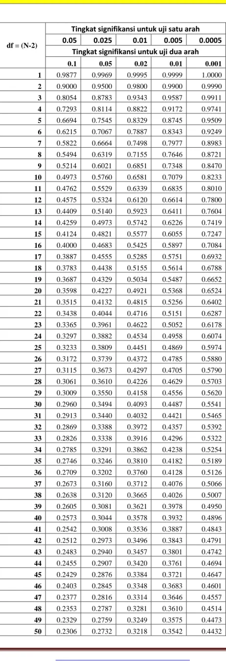
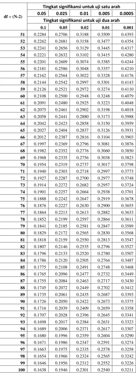
Dalam rangka uji validitas kuesioner kriteria pengujian, apabila r hitung > r tabel, dengan taraf signifikasi 0,05 dan df = n-2, maka alat ukur dinyatakan valid dan sebaliknya jika r hitung < r tabel maka item pertanyaan tersebut tidak valid. Petanyaan yang tidak valid tidak akan disertakan pada pengolahan data selanjutnya (Sugiyono, 2004).
Input Data Processing
Data Output
2
Uji Reliabilitas
dalah uji untuk memastikan apakah kuesioner penelitian yang akan dipergunakan untuk mengumpulkan data variable penelitian reliable atau tidak. Kuesioner dikatakan reliabel jika kuesioner tersebut dilakukan pengukuran ulang, maka akan mendapatkan hasil yang sama
Regresi Linear
Dalam regresi linear terdapat 2 jenis, yaitu : - Regresi Linear Sederhana
- Regresi Linear Berganda dan dalam tahap regresinya terdiri dari : a. Uji Asumsi Klasik
1. Uji Normalitas
Uji normalitas untuk menguji apakah nilai residual yang telah distandarisasi pada model regresi berdistribusi normal atau tidak. Cara melakukan uji normalitas dapat dilakukan dengan pendekatan analisis grafik normal probability Plot. Pada pendekatan ini nilai residual terdistribusi secara normal apabila garis (titik-titik) yang menggambarkan data sesungguhnya akan mengikuti atau merapat ke garis diagonalnya.
2. Uji Multikolinearitas
Uji multikolinearitas bertujuan untuk menguji apakah model regresi terbentuk adanya korelasi tinggi atau sempurna antar variabel bebas (independen). Jika ditemukan ada hubungan korelasi yang tinggi antar variabel bebas maka dapat dinyatakan adanya gejala multikorlinear pada penelitian.
3. Uji Autokorelasi
Uji autokolerasi merupakan kolerasi yang terjadi antara residual pada satu pengamatan dengan pengamatan lain pada model regresi. Autokorelasi dapat diketahui melalui Uji Durbin-Watson (D-W Test), adalah pengujian yang digunakan untuk menguji ada atau tidak adanya korelasi serial dalam model regresi atau untuk mengetahui apakah di dalam model yang digunakan terdapat autokorelasi diantara variabel-variabel yang diamati
4. Uji Heteroskedastisitas
Uji heteroskedastisitas digunakan untuk mengetahui ada atau tidaknya penyimpangan asumsi klasik.
Heteroskedastisitas yaitu adanya ketidaksamaan varian dari residual untuk semua pengamatan pada model regresi. Prasyarat yang harus terpenuhi dalam model regresi adalah tidak adanya gejala heteroskedastisitas.
b. Uji Kelayakan Model (Goodness of Fit)
3
Uji kelayakan model adalah uji R 2 untuk melihat kemampuan variable independen dalam menjelaskan variable dependen. Nilai R 2 berkisar antara 0 – 99, nilai R Square yang semakin mendekati 1 maka semakin layak suatu model untuk digunakan.
c. Uji Parsial (Uji t)
Uji partial (uji t) adalah uji yang dilakukan untuk melihat apakah suatu variable independen berpengaruh atau tidak terhadap variable dependen dengan membandingkan nilai t hitung dengan t tabel .
Kriteria pengujian uji t adalah sebagai berikut :
- Jika nilai t hitung > t tabel maka hipotesis di tolak, artinya variable tersebut berpengaruh terhadap variable dependen.
- Jika nilai t hitung < t tabel maka hipotesis di terima, artinya variable tersebut tidak berpengaruh terhadap variable dependen.
d. Uji Simultan (Uji F)
Uji Simultan (uji F) adalah uji yang dilakukan untuk melihat apakah semua variable independen secara bersama-sama berpengaruh atau tidak terhadap variable dependen dengan membandingkan nilai F hitung dengan F tabel .
- Jika nilai F hitung > F tabel maka hipotesis di tolak, artinya secara bersama-sama variable independen tersebut berpengaruh terhadap variable dependen.
- Jika nilai F hitung < F tabel maka hipotesis di terima, artinya secara bersama-sama variable independen tersebut tidak berpengaruh terhadap variable dependen.
Regresi Linear Sederhana
Regresi linear sederhana adalah regresi linear yang terdiri dari 1 variabel dependen (Y) dan 1 variabel independen (X).
Y t =β 0 + β 1 X1 t + ε t
Dimana :
Y : Variabel Dependen X : Variabel Independen ε : error term (Standar Error)
t : menunjukkan jenis data berupa data runtun waktu (Time Series)
Uji-uji yang perlu dilakukan :
4
- Uji Normalitas - Uji Autokorelasi - Uji Heteroskedastistas
“ Uji Multikolinearitas TIDAK dilakukan dalam regresi liear sederhana karena hanya terdiri dari 1
variabel independen”.
5
Uji Validitas
Cara menguji validitas dan realibilitas kuesioner dengan menggunakan spss 1. buka program spss
2. copy dan pastekan data yang terlebih dahulu diketik pada excel
6
3. setelah selesai di input, kemudian klik variabel view, pada kolom label, silahkan beri nama, misalnya
"X11,X12,X13,X14,X15,X16,Total X1 “
7
4. untuk uji validitas, klik menu analyze => correlate => bivariate
8
5. blok semua item x11 sampai x1 total dan masukan ke dalam kolom sebelah kanan, centang pada
"Pearson" dan "two-tailed" kemudian klik Ok
9
6. Hasil Uji validitas variabel X1
Karena unutk menentukkan valid atau tidaknya butir kuesioner, dilakukan dengan membandingkan nilai r thitung dan r tabel.
Jika r hitung < r tabel = tidak valid Jikar r hitung > r tabel = valid
Cara menentukkan r tabel adalah df = N-2, dimana N adalah jumlah sampel. Jadi sampel yang digunakan adalah sebanyak 100 sampel maka df=100-2, => df=98. Nilai r tabel dari df=98 adalah 0,196
dari hasil uji validitas dia tas dapat dilihat bahwa semua nila r hitung > dari 0,196 sehingga dapat disimpulkan semua butir kuesioner untuk variabel X1 adalah valid.
Uji Reliabilitas
Kategori koefisien reliabilitas (Guilford, 1956: 145) adalah sebagai berikut:
0,80 < r11 1,00 reliabilitas sangat tinggi 0,60 < r11 0,80 reliabilitas tinggi
0,40 < r11 0,60 reliabilitas sedang 0,20 < r11 0,40 reliabilitas rendah.
-1,00 r11 0,20 reliabilitas sangat rendah (tidak reliable).
10
7. selanjutnya uji reliabilitas, klik analyze => scale => Reliability test
8. masukan semua variabel pada kotak kiri ke kotak kanan, kecuali variabel "Total X1” kemudian klik OK
8. dari hasil uji reliabilitas, yang dilihat adalah nilai cronbach's alpha, nilai cronbach's alpha yang kita
peroleh sebesar 0,805, artinya kuesioner yang kita buat sudah reliabel karena lebih besar dari nilai 0,60
sehingga daat disimpulkan kuesioner penelitian tersebut reliabel.
11
Regresi Linier Berganda
Regresi linear Berganda adalah regresi linear yang terdiri dari 1 variabel dependen (Y) dan minimal memiliki 2 variabel independen (X).
Y t =β 0 + β 1 X1+ β 1 X2+ ε Dimana :
Y : Variabel Dependen X1 : Variabel X1
X2 : Variabel X2
ε : error term (Standar Error)
Uji-uji yang perlu dilakukan : - Uji Normalitas
- Uji Multikolinearitas - Uji Autokorelasi - Uji Heteroskedastistas
Cara Melakukan Regresi Linear Berganda Dengan Menggunakan SPSS
Buka file microsoft excel yang berisi data penelitian
Data yang akan digunakan untuk regresi data linier berganda adalah ariabel Y X1 dan X2
Block semua data yang akan digunakan dalam penelitian
12
Copy, kemudian pastekan di jendela SPSS
Setelah data dicopy, selanjutnya beri nama variabel misalny Y, X1, X2
13
Caranya adalah, klik variable view pada kiri bawah jendela spss
Kemudian beri nama variabel sesuai keinginan
14
Klik menu analyze => regression => linear
Pada kotak dependent variable masukan variabel Y . Pada kotak independen variable masukan variabel X1 dan X2
Pada jendela Linear Regression terdapat ribbon menu berupa Statistics, Plots, Save, Options, Bootstrap. Namun yang sering digunakan untuk prosesing data hanya
Statistics, Plots, Save
15
Klik statistic => untuk regression coefficient centang (√) pada r square change, descriptive, part and partial correlation serta colinearity diagnostic dan durbin-watson, kemudian klik continue
klik plot, pilih dependent ke Y axis dan Zresid ke X axis, dan klik histogram serta normality plot, kemudian
klik Continue
16
17
Hasil Output Regresi
18
Uji Asumsi Klasik
19
Uji Normalitas
Cara menguji normalitas data dengan Analisis Grafik 1. buka spss
2. input data yang digunakan 3. klik analyze, regression, linear
4. masukan Y ke dalam kotak dependen variabel, dan X1 dan X2 ke dalam kotak independen variable.
5. Klik pada menu "plots" .
6. Pada jendela plots, pilih dependent untuk Y, dan *ZRESID untuk X
7. Pada Standardized Residual Plots, centang histogram dan probability plots, klik continue
8. output yang dihasilkan sebagai berikut , abaikan hasil regrssi lainnya, cukup dilihat pada bagian "Chart"
saja
dari hasil gambar pertama dapat dilihat bahwa kurva dependen dan rss membentuk gambar seperti lonceng yang seimbang sehingga dapat disimpulkan bahwa data terdistribusi normal
dari gambar yang kedua dapat kita lihat bahwa titik2 persebaran data berada disekitar garis, hal ini menunjukkan bahwa data terdistribusi scara normal.
Uji Normalitas dengan Metode K-S (Kolomogrov-Smirnov)
Cara menguji normalitas data dengan Kolmogrov-Smirnov (K-S)
1. buka spss
20
2. input data yang digunakan 3. klik analyze, regression, linear
4. masukan Y ke dalam kotak dependen variabel, dan X1 dan X2 ke dalam kotak independen variable
5. klik "save"
6. Pada bagian "residual" centang pilihan "Standarized", kemudian klik continue 7. abaikan hasil outputnya, kemudian lihat pada jendela input,
pada data view, sudah ada variabel baru, yaitu "ZRE_1"
5. klik menu Analyze,=> Nonparametric Test => Legacy Dialog => 1 sample K-S 6. Masukan variabel "Standarized Residual" tersebut ke dalam ke kotak sebelah kanan
10. Maka hasilnya akan seperti berikut
Nilai residual terstandarisasi dalam penelitian tersebut menyebar secara normal, hal ini dapat dilihat dari nilai "Asymp. Sig. (2-tailed)" lebih besar dari 0,05
Uji Multikolineritas
Coefficients
aModel
Unstandardized Coefficients Standardized Coefficients
t Sig.
Correlations Collinearity Statistics
B Std. Error Beta Zero-order Partial Part Tolerance VIF
1 (Constant) 5.194 2.436 2.132 .035
X1 .449 .117 .434 3.841 .000 .717 .363 .259 .356 2.808
X2 .795 .254 .353 3.129 .002 .702 .303 .211 .356 2.808
a. Dependent Variable: Y
Dari nilai VIF di atas dapat dilihat bahwa nilai VIF X1 =2.808, VIF X2 = 2.808. Karena nilai VIF semua
variable independen < 10 maka dapat disimpulkan tidak terjadi gejala multikolinearitas pada model penelitian.
21
Uji Autokorelasi
Uji autokolerasi merupakan kolerasi yang terjadi antara residual pada satu pengamatan dengan pengamatan lain pada model regresi. Autokorelasi dapat diketahui melalui Uji Durbin-Watson (D-W Test), adalah pengujian yang digunakan untuk menguji ada atau tidak adanya korelasi serial dalam model regresi atau untuk mengetahui apakah di dalam model yang digunakan terdapat autokorelasi diantara variabel-variabel yang diamati.
Model Summary
bModel R R Square
Adjusted R Square
Std. Error of the Estimate
Change Statistics
Durbin- Watson R Square
Change
F
Change df1 df2
Sig. F Change
1 .748
a.559 .550 2.51675 .559 61.549 2 97 .000 1.467
a. Predictors: (Constant), X2, X1
b. Dependent Variable:
Y
Abaikan hasil yang lainnya, fokus kepada tabel "model Summary dapat dilihat bahwa nilai DW dari model tersebut adalah sebesar 1,467.
cara mencari tabel D-W N = 100
k = 2
Bandingkan dengan nilai tabel D-W dalam model ini terdapat masalah autokorelasi karena nilainya jauh di bawah nilai tabel dw yaitu dL = 1.502 & dU = 1.582.
Uji Heteroskedastistas
Cara menguji Heteroskedastisitas data dengan Metode Park
1. buka spss
2. input data yang digunakan 3. klik analyze, regression, linear
4. masukan Y ke dalam kotak dependen variabel, dan X1 X2 ke dalam kotak independen variabel
5. klik save => pada kotak residual pilih unstandarized => continue => ok
22
6. Abaikan hasil outputnya, kemudian pilih menu Tranform => compute Variable
7. pada "target variable" isi dengan "ABSResid"
8. pada kotak "Numeric Expression" isi dengan ABS(RES_1) => ok 9. selanjutnya kita akan mengulangi langkah 3 dan 4
10. pada langkah ke 4, Y keluarkan dari kotak dependen var, dan masukan ABSRESID ke dalam kotak
dependen var
23
Abaikan hasil lainnya, cukup lihat Tabel "coefficients"
Coefficients
aModel
Unstandardized Coefficients
Standardized Coefficients
t Sig.
B Std. Error Beta
1 (Constant) 6.082 1.325 4.589 .000
X1 -.173 .064 -.438 -2.718 .008
X2 .138 .138 .161 1.001 .319
a. Dependent Variable: ABSRESID
dari tabel dapat dilihat nilai "sig", variabel X1 memiliki nilai Prob 0,008 < 0,005, sehingga dapat disimpulkan bahwa terjadi masalah heteroskedastisitas dalam model.
Uji Parsial (Uji t)
Uji t dilakukan untuk melihat pengaruh suatu variable independen terhadap variable dependen.
Dengan menggunakan hipotesis : Ho : Tidak Berpengaruh
Ha : Berpengaruh
Jika nilai t hitung < t table , artinya Ho diterima Jika nilai t hitung > t table , artinya Ho ditolak
Dengan jumlah n=100 maka nilai t tabel ya adalah n-1= df-1= 99, nilai t tabelnya adalah 1,660
24
Coefficients
aModel
Unstandardized Coefficients Standardized Coefficients
t Sig.
Correlations Collinearity Statistics
B Std. Error Beta Zero-order Partial Part Tolerance VIF
1 (Constant) 5.194 2.436 2.132 .035
X1 .449 .117 .434 3.841 .000 .717 .363 .259 .356 2.808
X2 .795 .254 .353 3.129 .002 .702 .303 .211 .356 2.808
a. Dependent Variable: Y
- Variabel X1 memiliki nilai t hitung (3,841) > t table ( 1.660) , artinya kurs berpengaruh terhadap Y - Variabel X2 memiliki nilai t hitung (3,129) > t table ( 1.660) , artinya Inflasi berpengaruh terhadap Y Uji Simultan (Uji F)
Uji simultan dilakuakn untuk melihat pengaruh variable independen secara bersama-sama terhadap variable dependen.
Nilai df1 = k-1 = 2-1= 1 df 2 = n-k = 100-2 = 98
Berdasarkan tabel F dengan nilai df 1 = 1 dan df 2 = 98 maka nilai F tabelnya adalah 3,94
ANOVA
bModel Sum of Squares df Mean Square F Sig.
1 Regression 779.707 2 389.854 61.549 .000
aResidual 614.403 97 6.334
Total 1394.110 99
a. Predictors: (Constant), X2, X1
b. Dependent Variable: Y
Dari hasil regresi di atas dapat dilihat bahwa nilai F hitung (61,549) > nilai F table (3,94), sehingga
dapat disimpulkan bahwa variable independen secara bersama-sama berpengaruh terhadap variable dependen.
25
Interpretasi Hasil
Persamaan regresi yang diperoleh adalah
Y = 5.194+ 0.449 + 0.795 Dari regresi di atas maka dapat di interpretasikan hasil penelelitian
- Nilai koefisien konstanta sebesar 5.194, artinya jika variable X1 dan X2 dianggap konstan maka Y akan meningkat sebesar 5.194.
- Nilai koefisien X1 sebesar 0.449, artinya jika X1 meningkat sebesar 1 unit maka Y akan meningkat sebesar 0,449 dengan asumsi variable lain tetap.
- Nilai koefisien X2 sebesar 0.795, artinya jika X2 meningkat sebesar 1 unit maka Y akan meningkat
sebesar 0,795 dengan asumsi variable lain tetap.
26
Daftar Pustaka
Ghazali, M. (2017). Metodologi Penelitian. Jakarta: Salemba Empat.
Gujarati, D. N., & Porter, D. C. (2013). Dasar-Dasar Ekonometrika. Jakarta: Salemba Empat.
Suliyanto. (2006). Ekonometrika Terapan, Teori dan Aplikasi dengan SPSS. Jakarta: Penerbit Andi.
27
LAMPIRAN
28
Correlations
X11 X12 X13 X14 X15 X16 X17 X18 X19 X10 X1_TOTAL X11 Pearson Correlation 1 .466
**.377
**.215
*.175 .153 .037 .120 .347
**.268
**.504
**Sig. (2-tailed) .000 .000 .032 .082 .129 .711 .233 .000 .007 .000
N 100 100 100 100 100 100 100 100 100 100 100
X12 Pearson Correlation .466
**1 .613
**.331
**.130 .091 .061 .243
*.346
**.424
**.619
**Sig. (2-tailed) .000 .000 .001 .199 .366 .548 .015 .000 .000 .000
N 100 100 100 100 100 100 100 100 100 100 100
X13 Pearson Correlation .377
**.613
**1 .564
**.230
*.132 .177 .258
**.375
**.367
**.682
**Sig. (2-tailed) .000 .000 .000 .021 .190 .078 .010 .000 .000 .000
N 100 100 100 100 100 100 100 100 100 100 100
X14 Pearson Correlation .215
*.331
**.564
**1 .480
**.282
**.246
*.198
*.318
**.348
**.658
**Sig. (2-tailed) .032 .001 .000 .000 .004 .013 .048 .001 .000 .000
N 100 100 100 100 100 100 100 100 100 100 100
X15 Pearson Correlation .175 .130 .230
*.480
**1 .568
**.352
**.254
*.237
*.183 .577
**Sig. (2-tailed) .082 .199 .021 .000 .000 .000 .011 .017 .069 .000
N 100 100 100 100 100 100 100 100 100 100 100
X16 Pearson Correlation .153 .091 .132 .282
**.568
**1 .594
**.246
*.074 .115 .514
**Sig. (2-tailed) .129 .366 .190 .004 .000 .000 .014 .462 .256 .000
N 100 100 100 100 100 100 100 100 100 100 100
X17 Pearson Correlation .037 .061 .177 .246
*.352
**.594
**1 .430
**.119 .231
*.526
**Sig. (2-tailed) .711 .548 .078 .013 .000 .000 .000 .239 .021 .000
N 100 100 100 100 100 100 100 100 100 100 100
X18 Pearson Correlation .120 .243
*.258
**.198
*.254
*.246
*.430
**1 .353
**.418
**.594
**Sig. (2-tailed) .233 .015 .010 .048 .011 .014 .000 .000 .000 .000
N 100 100 100 100 100 100 100 100 100 100 100
X19 Pearson Correlation .347
**.346
**.375
**.318
**.237
*.074 .119 .353
**1 .572
**.648
**Sig. (2-tailed) .000 .000 .000 .001 .017 .462 .239 .000 .000 .000
N 100 100 100 100 100 100 100 100 100 100 100
X10 Pearson Correlation .268
**.424
**.367
**.348
**.183 .115 .231
*.418
**.572
**1 .687
**Sig. (2-tailed) .007 .000 .000 .000 .069 .256 .021 .000 .000 .000
N 100 100 100 100 100 100 100 100 100 100 100
X1_TOTAL Pearson Correlation .504
**.619
**.682
**.658
**.577
**.514
**.526
**.594
**.648
**.687
**1
Sig. (2-tailed) .000 .000 .000 .000 .000 .000 .000 .000 .000 .000
29
Reliability Statistics
Cronbach's
Alpha N of Items
.805 10
Variabel X2
Correlations
X21 X22 X23 X24 X2_TOTAL
X21 Pearson Correlation 1 .564
**.230
*.356
**.758
**Sig. (2-tailed) .000 .021 .000 .000
N 100 100 100 100 100
X22 Pearson Correlation .564
**1 .480
**.204
*.781
**Sig. (2-tailed) .000 .000 .041 .000
N 100 100 100 100 100
X23 Pearson Correlation .230
*.480
**1 .384
**.704
**Sig. (2-tailed) .021 .000 .000 .000
N 100 100 100 100 100
X24 Pearson Correlation .356
**.204
*.384
**1 .660
**Sig. (2-tailed) .000 .041 .000 .000
N 100 100 100 100 100
X2_TOTAL Pearson Correlation .758
**.781
**.704
**.660
**1
Sig. (2-tailed) .000 .000 .000 .000
N 100 100 100 100 100
**. Correlation is significant at the 0.01 level (2-tailed).
*. Correlation is significant at the 0.05 level (2-tailed).
Reliability Statistics
Cronbach's
Alpha N of Items
.702 4
N 100 100 100 100 100 100 100 100 100 100 100
**. Correlation is significant at the 0.01 level (2-tailed).
*. Correlation is significant at the 0.05 level (2-tailed).
30
Variabel Y
31
Correlations
Y1 Y2 Y3 Y4 Y5 Y6 Y7 Y8 Y9 Y_TOTAL Y1 Pearson Correlation 1 .805
**.590
**.407
**.251
*.360
**.399
**.471
**.507
**.761
**Sig. (2-tailed) .000 .000 .000 .012 .000 .000 .000 .000 .000
N 100 100 100 100 100 100 100 100 100 100
Y2 Pearson Correlation .805
**1 .696
**.464
**.253
*.301
**.304
**.518
**.519
**.776
**Sig. (2-tailed) .000 .000 .000 .011 .002 .002 .000 .000 .000
N 100 100 100 100 100 100 100 100 100 100
Y3 Pearson Correlation .590
**.696
**1 .633
**.412
**.311
**.162 .444
**.510
**.762
**Sig. (2-tailed) .000 .000 .000 .000 .002 .108 .000 .000 .000
N 100 100 100 100 100 100 100 100 100 100
Y4 Pearson Correlation .407
**.464
**.633
**1 .572
**.466
**.251
*.374
**.375
**.717
**Sig. (2-tailed) .000 .000 .000 .000 .000 .012 .000 .000 .000
N 100 100 100 100 100 100 100 100 100 100
Y5 Pearson Correlation .251
*.253
*.412
**.572
**1 .528
**.232
*.277
**.398
**.612
**Sig. (2-tailed) .012 .011 .000 .000 .000 .020 .005 .000 .000
N 100 100 100 100 100 100 100 100 100 100
Y6 Pearson Correlation .360
**.301
**.311
**.466
**.528
**1 .426
**.318
**.267
**.614
**Sig. (2-tailed) .000 .002 .002 .000 .000 .000 .001 .007 .000
N 100 100 100 100 100 100 100 100 100 100
Y7 Pearson Correlation .399
**.304
**.162 .251
*.232
*.426
**1 .491
**.427
**.568
**Sig. (2-tailed) .000 .002 .108 .012 .020 .000 .000 .000 .000
N 100 100 100 100 100 100 100 100 100 100
Y8 Pearson Correlation .471
**.518
**.444
**.374
**.277
**.318
**.491
**1 .800
**.747
**Sig. (2-tailed) .000 .000 .000 .000 .005 .001 .000 .000 .000
N 100 100 100 100 100 100 100 100 100 100
Y9 Pearson Correlation .507
**.519
**.510
**.375
**.398
**.267
**.427
**.800
**1 .768
**Sig. (2-tailed) .000 .000 .000 .000 .000 .007 .000 .000 .000
N 100 100 100 100 100 100 100 100 100 100
Y_TOTAL Pearson Correlation .761
**.776
**.762
**.717
**.612
**.614
**.568
**.747
**.768
**1 Sig. (2-tailed) .000 .000 .000 .000 .000 .000 .000 .000 .000
N 100 100 100 100 100 100 100 100 100 100
**. Correlation is significant at the 0.01 level (2-tailed).
*. Correlation is significant at the 0.05 level (2-tailed).
32
Reliability Statistics Cronbach's
Alpha N of Items
.874 9
Regresi Linear berganda
Descriptive Statistics
Mean Std. Deviation N
Y 31.6700 3.75259 100
X1 34.4700 3.62220 100
X2 13.8100 1.66785 100
Model Summary
bModel R R Square
Adjusted R Square
Std. Error of the Estimate
Change Statistics
Durbin- Watson R Square
Change
F
Change df1 df2
Sig. F Change
1 .748
a.559 .550 2.51675 .559 61.549 2 97 .000 1.467
a. Predictors: (Constant), X2, X1 b. Dependent Variable:
Y
ANOVA
bModel Sum of Squares df Mean Square F Sig.
1 Regression 779.707 2 389.854 61.549 .000
aResidual 614.403 97 6.334
Total 1394.110 99
a. Predictors: (Constant), X2, X1
b. Dependent Variable: Y
33
Coefficients
aModel
Unstandardized Coefficients Standardized Coefficients
t Sig.
Correlations Collinearity Statistics
B Std. Error Beta Zero-order Partial Part Tolerance VIF
1 (Constant) 5.194 2.436 2.132 .035
X1 .449 .117 .434 3.841 .000 .717 .363 .259 .356 2.808
X2 .795 .254 .353 3.129 .002 .702 .303 .211 .356 2.808
a. Dependent Variable: Y
34
1
A p p e n d i x
A
Durbin-Watson
Significance Tables
The Durbin-Watson test statistic tests the null hypothesis that the residuals from an ordinary least-squares regression are not autocorrelated against the alternative that the residuals follow an AR1 process. The Durbin-Watson statistic ranges in value from 0 to 4. A value near 2 indicates non-autocorrelation; a value toward 0 indicates positive autocorrelation; a value toward 4 indicates negative autocorrelation.
Because of the dependence of any computed Durbin-Watson value on the associated data matrix, exact critical values of the Durbin-Watson statistic are not tabulated for all possible cases. Instead, Durbin and Watson established upper and lower bounds for the critical values. Typically, tabulated bounds are used to test the hypothesis of zero autocorrelation against the alternative of positive first-order autocorrelation, since positive autocorrelation is seen much more frequently in practice than negative autocorrelation. To use the table, you must cross-reference the sample size against the number of regressors, excluding the constant from the count of the number of regressors.
The conventional Durbin-Watson tables are not applicable when you do not have a constant term in the regression. Instead, you must refer to an appropriate set of Durbin-Watson tables. The conventional Durbin-Watson tables are also not applicable when a lagged dependent variable appears among the regressors. Durbin has proposed alternative test procedures for this case.
Statisticians have compiled Durbin-Watson tables from some special cases, including:
Regressions with a full set of quarterly seasonal dummies.
Regressions with an intercept and a linear trend variable ( CURVEFIT MODEL=LINEAR ).
Regressions with a full set of quarterly seasonal dummies and a linear trend
variable.
2
Appendix A
In addition to obtaining the Durbin-Watson statistic for residuals from REGRESSION , you should also plot the ACF and PACF of the residuals series. The plots might suggest either that the residuals are random, or that they follow some ARMA process. If the residuals resemble an AR1 process, you can estimate an appropriate regression using the AREG procedure. If the residuals follow any ARMA process, you can estimate an appropriate regression using the ARIMA procedure.
In this appendix, we have reproduced two sets of tables. Savin and White (1977) present tables for sample sizes ranging from 6 to 200 and for 1 to 20 regressors for models in which an intercept is included. Farebrother (1980) presents tables for sample sizes ranging from 2 to 200 and for 0 to 21 regressors for models in which an intercept is not included.
Let’s consider an example of how to use the tables. In Chapter 9, we look at the classic Durbin and Watson data set concerning consumption of spirits. The sample size is 69, there are 2 regressors, and there is an intercept term in the model. The Durbin- Watson test statistic value is 0.24878. We want to test the null hypothesis of zero autocorrelation in the residuals against the alternative that the residuals are positively autocorrelated at the 1% level of significance. If you examine the Savin and White tables (Table A.2 and Table A.3), you will not find a row for sample size 69, so go to the next lowest sample size with a tabulated row, namely N=65. Since there are two regressors, find the column labeled k=2. Cross-referencing the indicated row and column, you will find that the printed bounds are dL = 1.377 and dU = 1.500. If the observed value of the test statistic is less than the tabulated lower bound, then you should reject the null hypothesis of non-autocorrelated errors in favor of the hypothesis of positive first-order autocorrelation. Since 0.24878 is less than 1.377, we reject the null hypothesis. If the test statistic value were greater than dU, we would not reject the null hypothesis.
A third outcome is also possible. If the test statistic value lies between dL and dU, the test is inconclusive. In this context, you might err on the side of conservatism and not reject the null hypothesis.
For models with an intercept, if the observed test statistic value is greater than 2, then you want to test the null hypothesis against the alternative hypothesis of negative first-order autocorrelation. To do this, compute the quantity 4-d and compare this value with the tabulated values of dL and dU as if you were testing for positive
autocorrelation.
When the regression does not contain an intercept term, refer to Farebrother’s
tabulated values of the “minimal bound,” denoted dM (Table A.4 and Table A.5),
instead of Savin and White’s lower bound dL. In this instance, the upper bound is
3 Durbin-Watson Significanc e Tables
the conventional bound dU found in the Savin and White tables. To test for negative first-order autocorrelation, use Table A.6 and Table A.7.
To continue with our example, had we run a regression with no intercept term, we
would cross-reference N equals 65 and k equals 2 in Farebrother’s table. The
tabulated 1% minimal bound is 1.348.
4
Appendix A
Table A-1
Models with an intercept (from Savin and White)
Durbin-Watson Statistic: 1 Per Cent Significance Points of dL and dU k’*=1
*k’ is the number of regressors excluding the intercept
k’=2 k’=3 k’=4 k’=5 k’=6 k’=7 k’=8 k’=9 k’=10
n dL dU dL dU dL dU dL dU dL dU dL dU dL dU dL dU dL dU dL dU
6 0.390 1.142 --- --- --- --- --- --- --- --- --- --- --- --- --- --- --- --- --- --- 7 0.435 1.036 0.294 1.676 --- --- --- --- --- --- --- --- --- --- --- --- --- --- --- --- 8 0.497 1.003 0.345 1.489 0.229 2.102 --- --- --- --- --- --- --- --- --- --- --- --- --- --- 9 0.554 0.998 0.408 1.389 0.279 1.875 0.183 2.433 --- --- --- --- --- --- --- --- --- --- --- --- 10 0.604 1.001 0.466 1.333 0.340 1.733 0.230 2.193 0.150 2.690 --- --- --- --- --- --- --- --- --- --- 11 0.653 1.010 0.519 1.297 0.396 1.640 0.286 2.030 0.193 2.453 0.124 2.892 --- --- --- --- --- --- --- --- 12 0.697 1.023 0.569 1.274 0.449 1.575 0.339 1.913 0.244 2.280 0.164 2.665 0.105 3.053 --- --- --- --- --- --- 13 0.738 1.038 0.616 1.261 0.499 1.526 0.391 1.826 0.294 2.150 0.211 2.490 0.140 2.838 0.090 3.182 --- --- --- --- 14 0.776 1.054 0.660 1.254 0.547 1.490 0.441 1.757 0.343 2.049 0.257 2.354 0.183 2.667 0.122 2.981 0.078 3.287 --- --- 15 0.811 1.070 0.700 1.252 0.591 1.465 0.487 1.705 0.390 1.967 0.303 2.244 0.226 2.530 0.161 2.817 0.107 3.101 0.068 3.374 16 0.844 1.086 0.738 1.253 0.633 1.447 0.532 1.664 0.437 1.901 0.349 2.153 0.269 2.416 0.200 2.681 0.142 2.944 0.094 3.201 17 0.873 1.102 0.773 1.255 0.672 1.432 0.574 1.631 0.481 1.847 0.393 2.078 0.313 2.319 0.241 2.566 0.179 2.811 0.127 3.053 18 0.902 1.118 0.805 1.259 0.708 1.422 0.614 1.604 0.522 1.803 0.435 2.015 0.355 2.238 0.282 2.467 0.216 2.697 0.160 2.925 19 0.928 1.133 0.835 1.264 0.742 1.416 0.650 1.583 0.561 1.767 0.476 1.963 0.396 2.169 0.322 2.381 0.255 2.597 0.196 2.813 20 0.952 1.147 0.862 1.270 0.774 1.410 0.684 1.567 0.598 1.736 0.515 1.918 0.436 2.110 0.362 2.308 0.294 2.510 0.232 2.174 21 0.975 1.161 0.889 1.276 0.803 1.408 0.718 1.554 0.634 1.712 0.552 1.881 0.474 2.059 0.400 2.244 0.331 2.434 0.268 2.625 22 0.997 1.174 0.915 1.284 0.832 1.407 0.748 1.543 0.666 1.691 0.587 1.849 0.510 2.015 0.437 2.188 0.368 2.367 0.304 2.548 23 1.017 1.186 0.938 1.290 0.858 1.407 0.777 1.535 0.699 1.674 0.620 1.821 0.545 1.977 0.473 2.140 0.404 2.308 0.340 2.479 24 1.037 1.199 0.959 1.298 0.881 1.407 0.805 1.527 0.728 1.659 0.652 1.797 0.578 1.944 0.507 2.097 0.439 2.255 0.375 2.417 25 1.055 1.210 0.981 1.305 0.906 1.408 0.832 1.521 0.756 1.645 0.682 1.776 0.610 1.915 0.540 2.059 0.473 2.209 0.409 2.362 26 1.072 1.222 1.000 1.311 0.928 1.410 0.855 1.517 0.782 1.635 0.711 1.759 0.640 1.889 0.572 2.026 0.505 2.168 0.441 2.313 27 1.088 1.232 1.019 1.318 0.948 1.413 0.878 1.514 0.808 1.625 0.738 1.743 0.669 1.867 0.602 1.997 0.536 2.131 0.473 2.269 28 1.104 1.244 1.036 1.325 0.969 1.414 0.901 1.512 0.832 1.618 0.764 1.729 0.696 1.847 0.630 1.970 0.566 2.098 0.504 2.229 29 1.119 1.254 1.053 1.332 0.988 1.418 0.921 1.511 0.855 1.611 0.788 1.718 0.723 1.830 0.658 1.947 0.595 2.068 0.533 2.193 30 1.134 1.264 1.070 1.339 1.006 1.421 0.941 1.510 0.877 1.606 0.812 1.707 0.748 1.814 0.684 1.925 0.622 2.041 0.562 2.160 31 1.147 1.274 1.085 1.345 1.022 1.425 0.960 1.509 0.897 1.601 0.834 1.698 0.772 1.800 0.710 1.906 0.649 2.017 0.589 2.131 32 1.160 1.283 1.100 1.351 1.039 1.428 0.978 1.509 0.917 1.597 0.856 1.690 0.794 1.788 0.734 1.889 0.674 1.995 0.615 2.104 33 1.171 1.291 1.114 1.358 1.055 1.432 0.995 1.510 0.935 1.594 0.876 1.683 0.816 1.776 0.757 1.874 0.698 1.975 0.641 2.080 34 1.184 1.298 1.128 1.364 1.070 1.436 1.012 1.511 0.954 1.591 0.896 1.677 0.837 1.766 0.779 1.860 0.722 1.957 0.665 2.057 35 1.195 1.307 1.141 1.370 1.085 1.439 1.028 1.512 0.971 1.589 0.914 1.671 0.857 1.757 0.800 1.847 0.744 1.940 0.689 2.037 36 1.205 1.315 1.153 1.376 1.098 1.442 1.043 1.513 0.987 1.587 0.932 1.666 0.877 1.749 0.821 1.836 0.766 1.925 0.711 2.018 37 1.217 1.322 1.164 1.383 1.112 1.446 1.058 1.514 1.004 1.585 0.950 1.662 0.895 1.742 0.841 1.825 0.787 1.911 0.733 2.001 38 1.227 1.330 1.176 1.388 1.124 1.449 1.072 1.515 1.019 1.584 0.966 1.658 0.913 1.735 0.860 1.816 0.807 1.899 0.754 1.985 39 1.237 1.337 1.187 1.392 1.137 1.452 1.085 1.517 1.033 1.583 0.982 1.655 0.930 1.729 0.878 1.807 0.826 1.887 0.774 1.970 40 1.246 1.344 1.197 1.398 1.149 1.456 1.098 1.518 1.047 1.583 0.997 1.652 0.946 1.724 0.895 1.799 0.844 1.876 0.749 1.956 45 1.288 1.376 1.245 1.424 1.201 1.474 1.156 1.528 1.111 1.583 1.065 1.643 1.019 1.704 0.974 1.768 0.927 1.834 0.881 1.902 50 1.324 1.403 1.285 1.445 1.245 1.491 1.206 1.537 1.164 1.587 1.123 1.639 1.081 1.692 1.039 1.748 0.997 1.805 0.955 1.864 55 1.356 1.428 1.320 1.466 1.284 1.505 1.246 1.548 1.209 1.592 1.172 1.638 1.134 1.685 1.095 1.734 1.057 1.785 1.018 1.837 60 1.382 1.449 1.351 1.484 1.317 1.520 1.283 1.559 1.248 1.598 1.214 1.639 1.179 1.682 1.144 1.726 1.108 1.771 1.072 1.817 65 1.407 1.467 1.377 1.500 1.346 1.534 1.314 1.568 1.283 1.604 1.251 1.642 1.218 1.680 1.186 1.720 1.153 1.761 1.120 1.802 70 1.429 1.485 1.400 1.514 1.372 1.546 1.343 1.577 1.313 1.611 1.283 1.645 1.253 1.680 1.223 1.716 1.192 1.754 1.162 1.792 75 1.448 1.501 1.422 1.529 1.395 1.557 1.368 1.586 1.340 1.617 1.313 1.649 1.284 1.682 1.256 1.714 1.227 1.748 1.199 1.783 80 1.465 1.514 1.440 1.541 1.416 1.568 1.390 1.595 1.364 1.624 1.338 1.653 1.312 1.683 1.285 1.714 1.259 1.745 1.232 1.777 85 1.481 1.529 1.458 1.553 1.434 1.577 1.411 1.603 1.386 1.630 1.362 1.657 1.337 1.685 1.312 1.714 1.287 1.743 1.262 1.773 90 1.496 1.541 1.474 1.563 1.452 1.587 1.429 1.611 1.406 1.636 1.383 1.661 1.360 1.687 1.336 1.714 1.312 1.741 1.288 1.769 95 1.510 1.552 1.489 1.573 1.468 1.596 1.446 1.618 1.425 1.641 1.403 1.666 1.381 1.690 1.358 1.715 1.336 1.741 1.313 1.767 100 1.522 1.562 1.502 1.582 1.482 1.604 1.461 1.625 1.441 1.647 1.421 1.670 1.400 1.693 1.378 1.717 1.357 1.741 1.335 1.765 150 1.611 1.637 1.598 1.651 1.584 1.665 1.571 1.679 1.557 1.693 1.543 1.708 1.530 1.722 1.515 1.737 1.501 1.752 1.486 1.767 200 1.664 1.684 1.653 1.693 1.643 1.704 1.633 1.715 1.623 1.725 1.613 1.735 1.603 1.746 1.592 1.757 1.582 1.768 1.571 1.779
5 Durbin-Watson Significanc e Tables
k’*=11
*k’ is the number of regressors excluding the intercept
k’=12 k’=13 k’=14 k’=15 k’=16 k’=17 k’=18 k’=19 k’=20
n dL dU dL dU dL dU dL dU dL dU dL dU dL dU dL dU dL dU dL dU 16 0.060 3.446 --- --- --- --- --- --- --- --- --- --- --- --- --- --- --- --- --- --- 17 0.084 3.286 0.053 3.506 --- --- --- --- --- --- --- --- --- --- --- --- --- --- --- --- 18 0.113 3.146 0.075 3.358 0.047 3.557 --- --- --- --- --- --- --- --- --- --- --- --- --- --- 19 0.145 3.023 0.102 3.227 0.067 3.420 0.043 3.601 --- --- --- --- --- --- --- --- --- --- --- --- 20 0.178 2.914 0.131 3.109 0.092 3.297 0.061 3.474 0.038 3.639 --- --- --- --- --- --- --- --- --- --- 21 0.212 2.817 0.162 3.004 0.119 3.185 0.084 3.358 0.055 3.521 0.035 3.671 --- --- --- --- --- --- --- --- 22 0.246 2.729 0.194 2.909 0.148 3.084 0.109 3.252 0.077 3.412 0.050 3.562 0.032 3.700 --- --- --- --- --- --- 23 0.281 2.651 0.227 2.822 0.178 2.991 0.136 3.155 0.100 3.311 0.070 3.459 0.046 3.597 0.029 3.725 --- --- --- --- 24 0.315 2.580 0.260 2.744 0.209 2.906 0.165 3.065 0.125 3.218 0.092 3.363 0.065 3.501 0.043 3.629 0.027 3.747 --- --- 25 0.348 2.517 0.292 2.674 0.240 2.829 0.194 2.982 0.152 3.131 0.116 3.274 0.085 3.410 0.060 3.538 0.039 3.657 0.025 3.766 26 0.381 2.460 0.324 2.610 0.272 2.758 0.224 2.906 0.180 3.050 0.141 3.191 0.107 3.325 0.079 3.452 0.055 3.572 0.036 3.682 27 0.413 2.409 0.356 2.552 0.303 2.694 0.253 2.836 0.208 2.976 0.167 3.113 0.131 3.245 0.100 3.371 0.073 3.490 0.051 3.602 28 0.444 2.363 0.387 2.499 0.333 2.635 0.283 2.772 0.237 2.907 0.194 3.040 0.156 3.169 0.122 3.294 0.093 3.412 0.068 3.524 29 0.474 2.321 0.417 2.451 0.363 2.582 0.313 2.713 0.266 2.843 0.222 2.972 0.182 3.098 0.146 3.220 0.114 3.338 0.087 3.450 30 0.503 2.283 0.447 2.407 0.393 2.533 0.342 2.659 0.294 2.785 0.249 2.909 0.208 3.032 0.171 3.152 0.137 3.267 0.107 3.379 31 0.531 2.248 0.475 2.367 0.422 2.487 0.371 2.609 0.322 2.730 0.277 2.851 0.234 2.970 0.193 3.087 0.160 3.201 0.128 3.311 32 0.558 2.216 0.503 2.330 0.450 2.446 0.399 2.563 0.350 2.680 0.304 2.797 0.261 2.912 0.221 3.026 0.184 3.137 0.151 3.246 33 0.585 2.187 0.530 2.296 0.477 2.408 0.426 2.520 0.377 2.633 0.331 2.746 0.287 2.858 0.246 2.969 0.209 3.078 0.174 3.184 34 0.610 2.160 0.556 2.266 0.503 2.373 0.452 2.481 0.404 2.590 0.357 2.699 0.313 2.808 0.272 2.915 0.233 3.022 0.197 3.126 35 0.634 2.136 0.581 2.237 0.529 2.340 0.478 2.444 0.430 2.550 0.383 2.655 0.339 2.761 0.297 2.865 0.257 2.969 0.221 3.071 36 0.658 2.113 0.605 2.210 0.554 2.310 0.504 2.410 0.455 2.512 0.409 2.614 0.364 2.717 0.322 2.818 0.282 2.919 0.244 3.019 37 0.680 2.092 0.628 2.186 0.578 2.282 0.528 2.379 0.480 2.477 0.434 2.576 0.389 2.675 0.347 2.774 0.306 2.872 0.268 2.969 38 0.702 2.073 0.651 2.164 0.601 2.256 0.552 2.350 0.504 2.445 0.458 2.540 0.414 2.637 0.371 2.733 0.330 2.828 0.291 2.923 39 0.723 2.055 0.673 2.143 0.623 2.232 0.575 2.323 0.528 2.414 0.482 2.507 0.438 2.600 0.395 2.694 0.354 2.787 0.315 2.879 40 0.744 2.039 0.694 2.123 0.645 2.210 0.597 2.297 0.551 2.386 0.505 2.476 0.461 2.566 0.418 2.657 0.377 2.748 0.338 2.838 45 0.835 1.972 0.790 2.044 0.744 2.118 0.700 2.193 0.655 2.269 0.612 2.346 0.570 2.424 0.528 2.503 0.488 2.582 0.448 2.661 50 0.913 1.925 0.871 1.987 0.829 2.051 0.787 2.116 0.746 2.182 0.705 2.250 0.665 2.318 0.625 2.387 0.586 2.456 0.548 2.526 55 0.979 1.891 0.940 1.945 0.902 2.002 0.863 2.059 0.825 2.117 0.786 2.176 0.748 2.237 0.711 2.298 0.674 2.359 0.637 2.421 60 1.037 1.865 1.001 1.914 0.965 1.964 0.929 2.015 0.893 2.067 0.857 2.120 0.822 2.173 0.786 2.227 0.751 2.283 0.716 2.338 65 1.087 1.845 1.053 1.889 1.020 1.934 0.986 1.980 0.953 2.027 0.919 2.075 0.886 2.123 0.852 2.172 0.819 2.221 0.789 2.272 70 1.131 1.831 1.099 1.870 1.068 1.911 1.037 1.953 1.005 1.995 0.974 2.038 0.943 2.082 0.911 2.127 0.880 2.172 0.849 2.217 75 1.170 1.819 1.141 1.856 1.111 1.893 1.082 1.931 1.052 1.970 1.023 2.009 0.993 2.049 0.964 2.090 0.934 2.131 0.905 2.172 80 1.205 1.810 1.177 1.844 1.150 1.878 1.122 1.913 1.094 1.949 1.066 1.984 1.039 2.022 1.011 2.059 0.983 2.097 0.955 2.135 85 1.236 1.803 1.210 1.834 1.184 1.866 1.158 1.898 1.132 1.931 1.106 1.965 1.080 1.999 1.053 2.033 1.027 2.068 1.000 2.104 90 1.264 1.798 1.240 1.827 1.215 1.856 1.191 1.886 1.166 1.917 1.141 1.948 1.116 1.979 1.091 2.012 1.066 2.044 1.041 2.077 95 1.290 1.793 1.267 1.821 1.244 1.848 1.221 1.876 1.197 1.905 1.174 1.943 1.150 1.963 1.126 1.993 1.102 2.023 1.079 2.054 100 1.314 1.790 1.292 1.816 1.270 1.841 1.248 1.868 1.225 1.895 1.203 1.922 1.181 1.949 1.158 1.977 1.136 2.006 1.113 2.034 150 1.473 1.783 1.458 1.799 1.444 1.814 1.429 1.830 1.414 1.847 1.400 1.863 1.385 1.880 1.370 1.897 1.355 1.913 1.340 1.931 200 1.561 1.791 1.550 1.801 1.539 1.813 1.528 1.824 1.518 1.836 1.507 1.847 1.495 1.860 1.484 1.871 1.474 1.883 1.462 1.896
6
Appendix A
Table A-2
Models with an intercept (from Savin and White)
Durbin-Watson Statistic: 5 Per Cent Significance Points of dL and dU k’*=1
*k’ is the number of regressors excluding the intercept
k’=2 k’=3 k’=4 k’=5 k’=6 k’=7 k’=8 k’=9 k’=10
n dL dU dL dU dL dU dL dU dL dU dL dU dL dU dL dU dL dU dL dU
6 0.610 1.400 --- --- --- --- --- --- --- --- --- --- --- --- --- --- --- --- --- --- 7 0.700 1.356 0.467 1.896 --- --- --- --- --- --- --- --- --- --- --- --- --- --- --- --- 8 0.763 1.332 0.559 1.777 0.367 2.287 --- --- --- --- --- --- --- --- --- --- --- --- --- --- 9 0.824 1.320 0.629 1.699 0.455 2.128 0.296 2.588 --- --- --- --- --- --- --- --- --- --- --- --- 10 0.879 1.320 0.697 1.641 0.525 2.016 0.376 2.414 0.243 2.822 --- --- --- --- --- --- --- --- --- --- 11 0.927 1.324 0.758 1.604 0.595 1.928 0.444 2.283 0.315 2.645 0.203 3.004 --- --- --- --- --- --- --- --- 12 0.971 1.331 0.812 1.579 0.658 1.864 0.512 2.177 0.380 2.506 0.268 2.832 0.171 3.149 --- --- --- --- --- --- 13 1.010 1.340 0.861 1.562 0.715 1.816 0.574 2.094 0.444 2.390 0.328 2.692 0.230 2.985 0.147 3.266 --- --- --- --- 14 1.045 1.350 0.905 1.551 0.767 1.779 0.632 2.030 0.505 2.296 0.389 2.572 0.286 2.848 0.200 3.111 0.127 3.360 --- --- 15 1.077 1.361 0.946 1.543 0.814 1.750 0.685 1.977 0.562 2.220 0.447 2.471 0.343 2.727 0.251 2.979 0.175 3.216 0.111 3.438 16 1.106 1.371 0.982 1.539 0.857 1.728 0.734 1.935 0.615 2.157 0.502 2.388 0.398 2.624 0.304 2.860 0.222 3.090 0.155 3.304 17 1.133 1.381 1.015 1.536 0.897 1.710 0.779 1.900 0.664 2.104 0.554 2.318 0.451 2.537 0.356 2.757 0.272 2.975 0.198 3.184 18 1.158 1.391 1.046 1.535 0.933 1.696 0.820 1.872 0.710 2.060 0.603 2.258 0.502 2.461 0.407 2.668 0.321 2.873 0.244 3.073 19 1.180 1.401 1.074 1.536 0.967 1.685 0.859 1.848 0.752 2.023 0.649 2.206 0.549 2.396 0.456 2.589 0.369 2.783 0.290 2.974 20 1.201 1.411 1.100 1.537 0.998 1.676 0.894 1.828 0.792 1.991 0.691 2.162 0.595 2.339 0.502 2.521 0.416 2.704 0.336 2.885 21 1.221 1.420 1.125 1.538 1.026 1.669 0.927 1.812 0.829 1.964 0.731 2.124 0.637 2.290 0.546 2.461 0.461 2.633 0.380 2.806 22 1.239 1.429 1.147 1.541 1.053 1.664 0.958 1.797 0.863 1.940 0.769 2.090 0.677 2.246 0.588 2.407 0.504 2.571 0.424 2.735 23 1.257 1.437 1.168 1.543 1.078 1.660 0.986 1.785 0.895 1.920 0.804 2.061 0.715 2.208 0.628 2.360 0.545 2.514 0.465 2.670 24 1.273 1.446 1.188 1.546 1.101 1.656 1.013 1.775 0.925 1.902 0.837 2.035 0.750 2.174 0.666 2.318 0.584 2.464 0.506 2.613 25 1.288 1.454 1.206 1.550 1.123 1.654 1.038 1.767 0.953 1.886 0.868 2.013 0.784 2.144 0.702 2.280 0.621 2.419 0.544 2.560 26 1.302 1.461 1.224 1.553 1.143 1.652 1.062 1.759 0.979 1.873 0.897 1.992 0.816 2.117 0.735 2.246 0.657 2.379 0.581 2.513 27 1.316 1.469 1.240 1.556 1.162 1.651 1.084 1.753 1.004 1.861 0.925 1.974 0.845 2.093 0.767 2.216 0.691 2.342 0.616 2.470 28 1.328 1.476 1.255 1.560 1.181 1.650 1.104 1.747 1.028 1.850 0.951 1.959 0.874 2.071 0.798 2.188 0.723 2.309 0.649 2.431 29 1.341 1.483 1.270 1.563 1.198 1.650 1.124 1.743 1.050 1.841 0.975 1.944 0.900 2.052 0.826 2.164 0.753 2.278 0.681 2.396 30 1.352 1.489 1.284 1.567 1.214 1.650 1.143 1.739 1.071 1.833 0.998 1.931 0.926 2.034 0.854 2.141 0.782 2.251 0.712 2.363 31 1.363 1.496 1.297 1.570 1.229 1.650 1.160 1.735 1.090 1.825 1.020 1.920 0.950 2.018 0.879 2.120 0.810 2.226 0.741 2.333 32 1.373 1.502 1.309 1.574 1.244 1.650 1.177 1.732 1.109 1.819 1.041 1.909 0.972 2.004 0.904 2.102 0.836 2.203 0.769 2.306 33 1.383 1.508 1.321 1.577 1.258 1.651 1.193 1.730 1.127 1.813 1.061 1.900 0.994 1.991 0.927 2.085 0.861 2.181 0.796 2.281 34 1.393 1.514 1.333 1.580 1.271 1.652 1.208 1.728 1.144 1.808 1.079 1.891 1.015 1.978 0.950 2.069 0.885 2.162 0.821 2.257 35 1.402 1.519 1.343 1.584 1.283 1.653 1.222 1.726 1.160 1.803 1.097 1.884 1.034 1.967 0.971 2.054 0.908 2.144 0.845 2.236 36 1.411 1.525 1.354 1.587 1.295 1.654 1.236 1.724 1.175 1.799 1.114 1.876 1.053 1.957 0.991 2.041 0.930 2.127 0.868 2.216 37 1.419 1.530 1.364 1.590 1.307 1.655 1.249 1.723 1.190 1.795 1.131 1.870 1.071 1.948 1.011 2.029 0.951 2.112 0.891 2.197 38 1.427 1.535 1.373 1.594 1.318 1.656 1.261 1.722 1.204 1.792 1.146 1.864 1.088 1.939 1.029 2.017 0.970 2.098 0.912 2.180 39 1.435 1.540 1.382 1.597 1.328 1.658 1.273 1.722 1.218 1.789 1.161 1.859 1.104 1.932 1.047 2.007 0.990 2.085 0.932 2.164 40 1.442 1.544 1.391 1.600 1.338 1.659 1.285 1.721 1.230 1.786 1.175 1.854 1.120 1.924 1.064 1.997 1.008 2.072 0.952 2.149 45 1.475 1.566 1.430 1.615 1.383 1.666 1.336 1.720 1.287 1.776 1.238 1.835 1.189 1.895 1.139 1.958 1.089 2.022 1.038 2.088 50 1.503 1.585 1.462 1.628 1.421 1.674 1.378 1.721 1.335 1.771 1.291 1.822 1.246 1.875 1.201 1.930 1.156 1.986 1.110 2.044 55 1.528 1.601 1.490 1.641 1.452 1.681 1.414 1.724 1.374 1.768 1.334 1.814 1.294 1.861 1.253 1.909 1.212 1.959 1.170 2.010 60 1.549 1.616 1.514 1.652 1.480 1.689 1.444 1.727 1.408 1.767 1.372 1.808 1.335 1.850 1.298 1.894 1.260 1.939 1.222 1.984 65 1.567 1.629 1.536 1.662 1.503 1.696 1.471 1.731 1.438 1.767 1.404 1.805 1.370 1.843 1.336 1.882 1.301 1.923 1.266 1.964 70 1.583 1.641 1.554 1.672 1.525 1.703 1.494 1.735 1.464 1.768 1.433 1.802 1.401 1.838 1.369 1.874 1.337 1.910 1.305 1.948 75 1.598 1.652 1.571 1.680 1.543 1.709 1.515 1.739 1.487 1.770 1.458 1.801 1.428 1.834 1.399 1.867 1.369 1.901 1.339 1.935 80 1.611 1.662 1.586 1.688 1.560 1.715 1.534 1.743 1.507 1.772 1.480 1.801 1.453 1.831 1.425 1.861 1.397 1.893 1.369 1.925 85 1.624 1.671 1.600 1.696 1.575 1.721 1.550 1.747 1.525 1.774 1.500 1.801 1.474 1.829 1.448 1.857 1.422 1.886 1.396 1.916 90 1.635 1.679 1.612 1.703 1.589 1.726 1.566 1.751 1.542 1.776 1.518 1.801 1.494 1.827 1.469 1.854 1.445 1.881 1.420 1.909 95 1.645 1.687 1.623 1.709 1.602 1.732 1.579 1.755 1.557 1.778 1.535 1.802 1.512 1.827 1.489 1.852 1.465 1.877 1.442 1.903 100 1.654 1.694 1.634 1.715 1.613 1.736 1.592 1.758 1.571 1.780 1.550 1.803 1.528 1.826 1.506 1.850 1.484 1.874 1.462 1.898 150 1.720 1.747 1.706 1.760 1.693 1.774 1.679 1.788 1.665 1.802 1.651 1.817 1.637 1.832 1.622 1.846 1.608 1.862 1.593 1.877 200 1.758 1.779 1.748 1.789 1.738 1.799 1.728 1.809 1.718 1.820 1.707 1.831 1.697 1.841 1.686 1.852 1.675 1.863 1.665 1.874
7 Durbin-Watson Significanc e Tables
k’*=11
*K’ is the number of regressors excluding the intercept
k’=12 k’=13 k’=14 k’=15 k’=16 k’=17 k’=18 k’=19 k’=20
n dL dU dL dU dL dU dL dU dL dU dL dU dL dU dL dU dL dU dL dU 16 0.098 3.503 --- --- --- --- --- --- --- --- --- --- --- --- --- --- --- --- --- --- 17 0.138 3.378 0.087 3.557 --- --- --- --- --- --- --- --- --- --- --- --- --- --- --- --- 18 0.177 3.265 0.123 3.441 0.078 3.603 --- --- --- --- --- --- --- --- --- --- --- --- --- --- 19 0.220 3.159 0.160 3.335 0.111 3.496 0.070 3.642 --- --- --- --- --- --- --- --- --- --- --- --- 20 0.263 3.063 0.200 3.234 0.145 3.395 0.100 3.542 0.063 3.676 --- --- --- --- --- --- --- --- --- --- 21 0.307 2.976 0.240 3.141 0.182 3.300 0.132 3.448 0.091 3.583 0.058 3.705 --- --- --- --- --- --- --- --- 22 0.349 2.897 0.281 3.057 0.220 3.211 0.166 3.358 0.120 3.495 0.083 3.619 0.052 3.731 --- --- --- --- --- --- 23 0.391 2.826 0.322 2.979 0.259 3.128 0.202 3.272 0.153 3.409 0.110 3.535 0.076 3.650 0.048 3.753 --- --- --- --- 24 0.431 2.761 0.362 2.908 0.297 3.053 0.239 3.193 0.186 3.327 0.141 3.454 0.101 3.572 0.070 3.678 0.044 3.773 --- --- 25 0.470 2.702 0.400 2.844 0.335 2.983 0.275 3.119 0.221 3.251 0.172 3.376 0.130 3.494 0.094 3.604 0.065 3.702 0.041 3.790 26 0.508 2.649 0.438 2.784 0.373 2.919 0.312 3.051 0.256 3.179 0.205 3.303 0.160 3.420 0.120 3.531 0.087 3.632 0.060 3.724 27 0.544 2.600 0.475 2.730 0.409 2.859 0.348 2.987 0.291 3.112 0.238 3.233 0.191 3.349 0.149 3.460 0.112 3.563 0.081 3.658 28 0.578 2.555 0.510 2.680 0.445 2.805 0.383 2.928 0.325 3.050 0.271 3.168 0.222 3.283 0.178 3.392 0.138 3.495 0.104 3.592 29 0.612 2.515 0.544 2.634 0.479 2.755 0.418 2.874 0.359 2.992 0.305 3.107 0.254 3.219 0.208 3.327 0.166 3.431 0.129 3.528 30 0.643 2.477 0.577 2.592 0.512 2.708 0.451 2.823 0.392 2.937 0.337 3.050 0.286 3.160 0.238 3.266 0.195 3.368 0.156 3.465 31 0.674 2.443 0.608 2.553 0.545 2.665 0.484 2.776 0.425 2.887 0.370 2.996 0.317 3.103 0.269 3.208 0.224 3.309 0.183 3.406 32 0.703 2.411 0.638 2.517 0.576 2.625 0.515 2.733 0.457 2.840 0.401 2.946 0.349 3.050 0.299 3.153 0.253 3.252 0.211 3.348 33 0.731 2.382 0.668 2.484 0.606 2.588 0.546 2.692 0.488 2.796 0.432 2.899 0.379 3.000 0.329 3.100 0.283 3.198 0.239 3.293 34 0.758 2.355 0.695 2.454 0.634 2.554 0.575 2.654 0.518 2.754 0.462 2.854 0.409 2.954 0.359 3.051 0.312 3.147 0.267 3.240 35 0.783 2.330 0.722 2.425 0.662 2.521 0.604 2.619 0.547 2.716 0.492 2.813 0.439 2.910 0.388 3.005 0.340 3.099 0.295 3.190 36 0.808 2.306 0.748 2.398 0.689 2.492 0.631 2.586 0.575 2.680 0.520 2.774 0.467 2.868 0.417 2.961 0.369 3.053 0.323 3.142 37 0.831 2.285 0.772 2.374 0.714 2.464 0.657 2.555 0.602 2.646 0.548 2.738 0.495 2.829 0.445 2.920 0.397 3.009 0.351 3.097 38 0.854 2.265 0.796 2.351 0.739 2.438 0.683 2.526 0.628 2.614 0.575 2.703 0.522 2.792 0.472 2.880 0.424 2.968 0.378 3.054 39 0.875 2.246 0.819 2.329 0.763 2.413 0.707 2.499 0.653 2.585 0.600 2.671 0.549 2.757 0.499 2.843 0.451 2.929 0.404 3.013 40 0.896 2.228 0.840 2.309 0.785 2.391 0.731 2.473 0.678 2.557 0.626 2.641 0.575 2.724 0.525 2.808 0.477 2.829 0.430 2.974 45 0.988 2.156 0.938 2.225 0.887 2.296 0.838 2.367 0.788 2.439 0.740 2.512 0.692 2.586 0.644 2.659 0.598 2.733 0.553 2.807 50 1.064 2.103 1.019 2.163 0.973 2.225 0.927 2.287 0.882 2.350 0.836 2.414 0.792 2.479 0.747 2.544 0.703 2.610 0.660 2.675 55 1.129 2.062 1.087 2.116 1.045 2.170 1.003 2.225 0.961 2.281 0.919 2.338 0.877 2.396 0.836 2.454 0.795 2.512 0.754 2.571 60 1.184 2.031 1.145 2.079 1.106 2.127 1.068 2.177 1.029 2.227 0.990 2.278 0.951 2.330 0.913 2.382 0.874 2.434 0.836 2.487 65 1.231 2.006 1.195 2.049 1.160 2.093 1.124 2.138 1.088 2.183 1.052 2.229 1.016 2.276 0.980 2.323 0.944 2.371 0.908 2.419 70 1.272 1.987 1.239 2.026 1.206 2.066 1.172 2.106 1.139 2.148 1.105 2.189 1.072 2.232 1.038 2.275 1.005 2.318 0.971 2.362 75 1.308 1.970 1.277 2.006 1.247 2.043 1.215 2.080 1.184 2.118 1.153 2.156 1.121 2.195 1.090 2.235 1.058 2.275 1.027 2.315 80 1.340 1.957 1.311 1.991 1.283 2.024 1.253 2.059 1.224 2.093 1.195 2.129 1.165 2.165 1.136 2.201 1.106 2.238 1.076 2.275 85 1.369 1.946 1.342 1.977 1.315 2.009 1.287 2.040 1.260 2.073 1.232 2.105 1.205 2.139 1.177 2.172 1.149 2.206 1.121 2.241 90 1.395 1.937 1.369 1.966 1.344 1.995 1.318 2.025 1.292 2.055 1.266 2.085 1.240 2.116 1.213 2.148 1.187 2.179 1.160 2.211 95 1.418 1.930 1.394 1.956 1.370 1.984 1.345 2.012 1.321 2.040 1.296 2.068 1.271 2.097 1.247 2.126 1.222 2.156 1.197 2.186 100 1.439 1.923 1.416 1.948 1.393 1.974 1.371 2.000 1.347 2.026 1.324 2.053 1.301 2.080 1.277 2.108 1.253 2.135 1.229 2.164 150 1.579 1.892 1.564 1.908 1.550 1.924 1.535 1.940 1.519 1.956 1.504 1.972 1.489 1.989 1.474 2.006 1.458 2.023 1.443 2.040 200 1.654 1.885 1.643 1.896 1.632 1.908 1.621 1.919 1.610 1.931 1.599 1.943 1.588 1.955 1.576 1.967 1.565 1.979 1.554 1.991
8
Appendix A
Table A-3
Models with no intercept (from Farebrother): Positive serial correlation
Durbin-Watson One Per Cent Minimal Bound
N K=0 K=1 K=2 K=3 K=4 K=5 K=6 K=7 K=8 K=9 K=10 K=11 K=12 K=13 K=14 K=15 K=16 K=17 K=18 K=19 K=20 K=21 2 0.001 --- --- --- --- --- --- --- --- --- --- --- --- --- --- --- --- --- --- --- --- --- 3 0.034 0.000 --- --- --- --- --- --- --- --- --- --- --- --- --- --- --- --- --- --- --- --- 4 0.127 0.022 0.000 --- --- --- --- --- --- --- --- --- --- --- --- --- --- --- --- --- --- --- 5 0.233 0.089 0.014 0.000 --- --- --- --- --- --- --- --- --- --- --- --- --- --- --- --- --- --- 6 0.322 0.175 0.065 0.010 0.000 --- --- --- --- --- --- --- --- --- --- --- --- --- --- --- --- --- 7 0.398 0.253 0.135 0.049 0.008 0.000 --- --- --- --- --- --- --- --- --- --- --- --- --- --- --- --- 8 0.469 0.324 0.202 0.106 0.038 0.006 0.000 --- --- --- --- --- --- --- --- --- --- --- --- --- --- --- 9 0.534 0.394 0.268 0.164 0.086 0.031 0.005 0.000 --- --- --- --- --- --- --- --- --- --- --- --- --- --- 10 0.591 0.457 0.333 0.223 0.136 0.070 0.025 0.004 0.000 --- --- --- --- --- --- --- --- --- --- --- --- --- 11 0.643 0.515 0.394 0.284 0.189 0.114 0.059 0.021 0.003 0.000 --- --- --- --- --- --- --- --- --- --- --- --- 12 0.691 0.568 0.451 0.341 0.244 0.161 0.097 0.050 0.018 0.003 0.000 --- --- --- --- --- --- --- --- --- --- --- 13 0.733 0.617 0.503 0.396 0.298 0.212 0.139 0.083 0.043 0.015 0.002 0.000 --- --- --- --- --- --- --- --- --- --- 14 0.773 0.662 0.552 0.448 0.350 0.262 0.185 0.121 0.072 0.037 0.013 0.002 0.000 --- --- --- --- --- --- --- --- --- 15 0.809 0.703 0.598 0.496 0.400 0.311 0.232 0.163 0.107 0.063 0.032 0.011 0.002 0.000 --- --- --- --- --- --- --- --- 16 0.842 0.741 0.640 0.541 0.447 0.358 0.278 0.206 0.145 0.094 0.056 0.028 0.010 0.002 0.000 --- --- --- --- --- --- --- 17 0.873 0.776 0.679 0.583 0.491 0.404 0.323 0.249 0.184 0.129 0.084 0.050 0.025 0.009 0.001 0.000 --- --- --- --- --- --- 18 0.901 0.808 0.715 0.623 0.533 0.447 0.366 0.292 0.225 0.166 0.116 0.075 0.044 0.023 0.008 0.001 0.000 --- --- --- --- --- 19 0.928 0.839 0.749 0.660 0.572 0.488 0.408 0.333 0.265 0.204 0.150 0.105 0.068 0.040 0.020 0.007 0.001 0.000 --- --- --- --- 20 0.952 0.867 0.780 0.694 0.609 0.527 0.448 0.374 0.304 0.241 0.185 0.136 0.095 0.062 0.036 0.018 0.006 0.001 0.000 --- --- --- 21 0.976 0.893 0.810 0.727 0.644 0.564 0.486 0.413 0.343 0.279 0.221 0.169 0.124 0.087 0.056 0.033 0.017 0.006 0.001 0.000 --- --- 22 0.997 0.918 0.838 0.757 0.677 0.599 0.523 0.450 0.381 0.316 0.257 0.203 0.155 0.114 0.079 0.051 0.030 0.015 0.005 0.001 0.000 --- 23 1.018 0.942 0.864 0.786 0.709 0.632 0.558 0.486 0.417 0.352 0.292 0.237 0.187 0.143 0.104 0.073 0.047 0.027 0.014 0.005 0.001 0.000 24 1.037 0.964 0.889 0.813 0.738 0.664 0.591 0.520 0.452 0.387 0.327 0.270 0.219 0.172 0.131 0.096 0.067 0.043 0.025 0.013 0.004 0.001 25 1.056 0.984 0.912 0.839 0.766 0.693 0.622 0.553 0.486 0.421 0.361 0.304 0.251 0.203 0.160 0.122 0.089 0.062 0.040 0.023 0.012 0.004 26 1.073 1.004 0.934 0.863 0.792 0.722 0.652 0.584 0.518 0.454 0.394 0.336 0.283 0.233 0.189 0.148 0.113 0.083 0.057 0.037 0.022 0.011 27 1.089 1.023 0.955 0.886 0.817 0.749 0.681 0.614 0.549 0.486 0.426 0.368 0.314 0.264 0.218 0.176 0.138 0.105 0.077 0.053 0.034 0.020 28 1.105 1.040 0.974 0.908 0.841 0.774 0.708 0.643 0.579 0.517 0.457 0.400 0.345 0.294 0.247 0.204 0.164 0.129 0.098 0.071 0.050 0.032 29 1.120 1.057 0.993 0.929 0.864 0.798 0.734 0.670 0.607 0.546 0.487 0.430 0.376 0.324 0.276 0.232 0.191 0.154 0.120 0.091 0.067 0.046 30 1.134 1.073 1.011 0.948 0.885 0.822 0.759 0.696 0.635 0.574 0.516 0.460 0.405 0.354 0.305 0.260 0.217 0.179 0.144 0.113 0.086 0.062 31 1.147 1.088 1.028 0.967 0.905 0.844 0.782 0.721 0.661 0.602 0.544 0.488 0.434 0.383 0.334 0.288 0.244 0.205 0.168 0.135 0.106 0.080 32 1.160 1.103 1.044 0.985 0.925 0.865 0.805 0.745 0.686 0.628 0.571 0.516 0.462 0.411 0.362 0.315 0.271 0.230 0.193 0.158 0.127 0.100 33 1.173 1.117 1.060 1.002 0.944 0.885 0.826 0.768 0.710 0.653 0.597 0.542 0.489 0.438 0.389 0.342 0.298 0.256 0.218 0.182 0.149 0.120 34 1.185 1.130 1.075 1.018 0.961 0.904 0.847 0.790 0.733 0.677 0.622 0.568 0.516 0.465 0.416 0.369 0.324 0.282 0.243 0.206 0.172 0.141 35 1.196 1.143 1.089 1.034 0.978 0.923 0.867 0.811 0.755 0.700 0.646 0.593 0.541 0.491 0.442 0.395 0.350 0.308 0.268 0.230 0.195 0.163 36 1.207 1.155 1.102 1.049 0.995 0.940 0.886 0.831 0.777 0.723 0.669 0.617 0.566 0.516 0.467 0.421 0.376 0.333 0.292 0.254 0.218 0.185 37 1.217 1.167 1.116 1.063 1.010 0.957 0.904 0.850 0.797 0.744 0.692 0.640 0.590 0.540 0.492 0.446 0.401 0.358 0.317 0.278 0.241 0.207 38 1.228 1.178 1.128 1.077 1.026 0.974 0.921 0.869 0.817 0.765 0.713 0.663 0.613 0.564 0.516 0.470 0.425 0.382 0.341 0.302 0.265 0.230 39 1.237 1.189 1.140 1.090 1.040 0.989 0.938 0.887 0.836 0.785 0.734 0.684 0.635 0.587 0.540 0.494 0.449 0.406 0.365 0.325 0.288 0.252 40 1.247 1.200 1.152 1.103 1.054 1.004 0.954 0.904 0.854 0.804 0.754 0.705 0.657 0.609 0.562 0.517 0.473 0.430 0.388 0.349 0.311 0.275 45 1.289 1.247 1.204 1.160 1.116 1.071 1.026 0.981 0.936 0.890 0.845 0.800 0.755 0.710 0.666 0.623 0.581 0.539 0.499 0.459 0.421 0.384 50 1.325 1.287 1.248 1.208 1.168 1.128 1.087 1.046 1.004 0.963 0.921 0.880 0.838 0.797 0.756 0.715 0.675 0.636 0.597 0.559 0.521 0.485 55 1.356 1.321 1.286 1.250 1.213 1.176 1.139 1.101 1.063 1.025 0.987 0.948 0.910 0.872 0.833 0.796 0.758 0.721 0.684 0.647 0.611 0.576 60 1.383 1.351 1.319 1.285 1.252 1.218 1.183 1.149 1.114 1.078 1.043 1.008 0.972 0.936 0.901 0.865 0.830 0.795 0.760 0.725 0.691 0.657 65 1.408 1.378 1.348 1.317 1.286 1.254 1.222 1.190 1.158 1.125 1.092 1.059 1.026 0.993 0.960 0.927 0.894 0.861 0.828 0.795 0.762 0.730 70 1.429 1.401 1.373 1.345 1.316 1.286 1.257 1.227 1.197 1.166 1.136 1.105 1.074 1.043 1.012 0.981 0.950 0.919 0.888 0.857 0.826 0.795 75 1.448 1.423 1.396 1.369 1.342 1.315 1.287 1.260 1.231 1.203 1.174 1.146 1.117 1.088 1.058 1.029 1.000 0.971 0.941 0.912 0.883 0.854 80 1.466 1.442 1.417 1.392 1.367 1.341 1.315 1.289 1.262 1.236 1.209 1.182 1.155 1.127 1.100 1.072 1.045 1.017 0.989 0.962 0.934 0.907 85 1.482 1.459 1.436 1.412 1.388 1.364 1.340 1.315 1.290 1.265 1.240 1.214 1.189 1.163 1.137 1.111 1.085 1.059 1.033 1.006 0.980 0.954 90 1.497 1.475 1.453 1.431 1.408 1.385 1.362 1.339 1.315 1.292 1.268 1.244 1.220 1.195 1.171 1.146 1.121 1.097 1.072 1.047 1.022 0.997 95 1.510 1.490 1.469 1.448 1.426 1.405 1.383 1.361 1.338 1.316 1.293 1.271 1.248 1.225 1.201 1.178 1.155 1.131 1.108 1.084 1.060 1.037 100 1.523 1.503 1.483 1.463 1.443 1.422 1.402 1.381 1.359 1.338 1.317 1.295 1.273 1.251 1.229 1.207 1.185 1.162 1.140 1.118 1.095 1.072 150 1.611 1.598 1.585 1.571 1.558 1.544 1.530 1.516 1.502 1.488 1.474 1.460 1.445 1.431 1.416 1.402 1.387 1.372 1.357 1.342 1.327 1.312 200 1.664 1.654 1.644 1.634 1.624 1.613 1.603 1.593 1.582 1.572 1.561 1.551 1.540 1.529 1.519 1.508 1.497 1.486 1.475 1.434 1.453 1.442