Another beauty of LBM is to deal with complex phenomena such as moving boundaries (multiphase, solidification and melting problems), obviously without the need for face tracking method as it is in the traditional CFD. The book is an introduction to the subject of LBM with emphasis on the applications and a few complete examples with computer codes are included in the text.
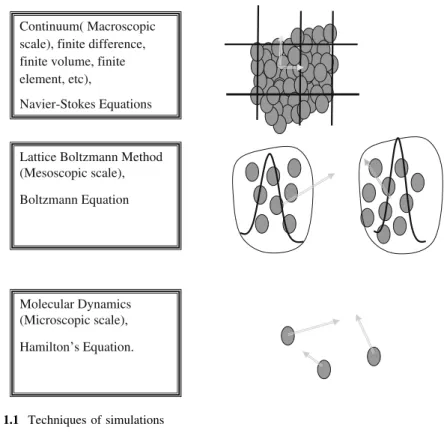
Introduction
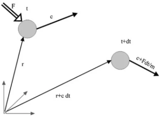
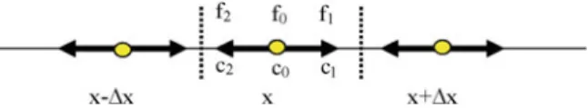
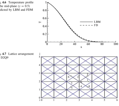
The question is whether we really need to know the behavior of every molecule or atom. In the bookkeeping process, we need to identify the location (x; y; z) and velocity (cx; cy; and cz are the components of velocity in the x; y and z directions) of each particle.
Kinetic Theory
Particle Dynamics
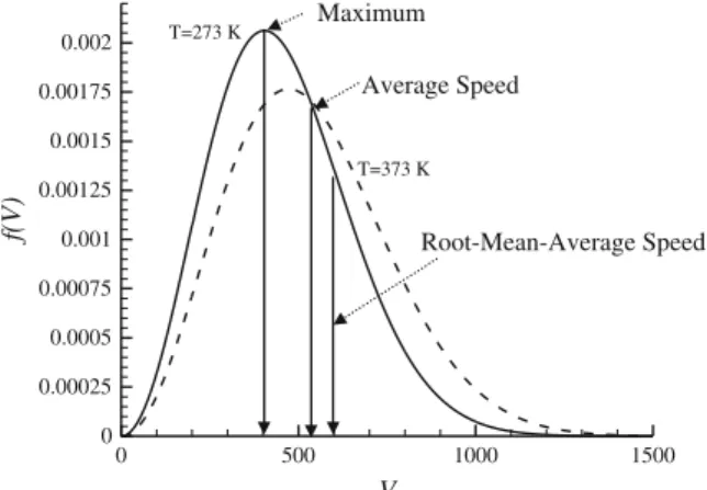
The magnitude of the particle velocity increases and the interaction between the particles increases as the internal energy of the system increases (for example, by heating the system). Increases in the kinetic energy of the molecules are called temperature increases in the macroscopic world.
Pressure and Temperature
This simple picture of molecular motion relates pressure in the macroscopic sense to the kinetic energy of molecules, i.e. KE¼mc2=2¼ ð3=2ÞkT ð1:12Þ Interestingly, temperature and pressure in the macroscopic world are no more than the rate of kinetic energy of molecules in the microscopic world.
Distribution Function
Boltzmann Distribution
For example, for a given energy, there are many more possible microscopic arrangements of gas molecules, with the gas essentially uniformly distributed in a box, than that of all the gas molecules located on the left half of the box. So if a liter of gas goes through all possible microscopic arrangements over time, there is essentially a negligible chance that it will all be in the left hemisphere at a time as old as the universe.
Boltzmann Transport Equation
Example 2.1
In a road intersection, if there are no car collisions, the cars from section A move (flow) to A0 and cars from section B move to B0 without any problem. However, if there is a collision at the intersection, cars at section A cannot move smoothly to A0 or from B to B0.
The BGKW Approximation
The beauty of this equation lies in its simplicity and can be applied to many physics simply by specifying a different equilibrium distribution function and source term (external force). It is possible to use finite difference or finite volume to solve partial differential equation (2.15).
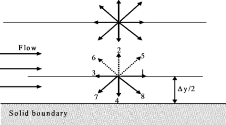
Lattice Arrangements
One-Dimensional
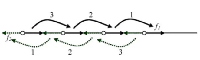
For this arrangement, the total number of actual particles cannot exceed three particles at any time. The other two particles move either to the left or to the right node in the stream process.
Two-Dimensional
For this arrangement, the total number of spurious particles at any time cannot exceed five particles. It is worth noting that this arrangement cannot be used to simulate fluid flows.
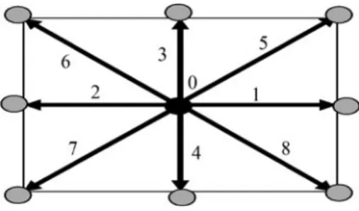
Three-Dimensional
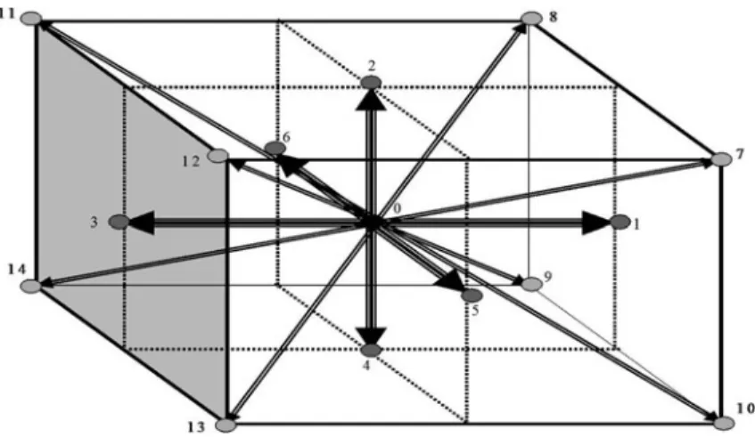
In this model, 15 velocity vectors are used, Fig.2.6, the central distribution function,f0 has zero speed. Note that nodes 1, 2, 3 and 4 are in the middle of the east, north, west and south planes respectively.
Equilibrium Distribution Function
Diffusion Equation
Example 3.1
The heat diffusion due to molecular action depends on the thermal conductivity (k), the density (q) and the specific heat (C). Therefore, the only parameter that controls the diffusion of heat is the thermal diffusivity of the medium, which is a property of the material.
Example 3.2
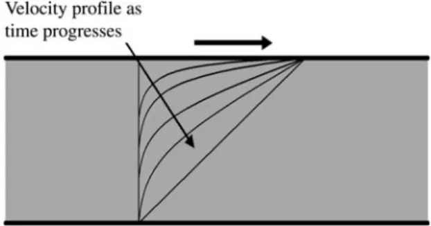
The time it takes for the lower plate to sense the movement of the upper plate depends on the viscosity of the fluid (high viscosity means less sensing time) and the distance between the plates (cf. 3.3).
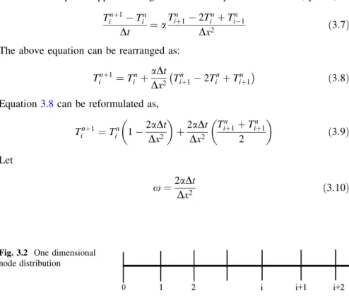
Finite Differences Approximation
The finite difference approximation for the diffusion equation is manipulation in the form of equation 3.11 to compare the finite difference formulation with LBM. Let's Eq. 3.11 studies, the last term (0:5½Tniþ1þTni1) is an average of temperatures around Ti: In other words, the average term represents the equilibrium value of Ti: Because Ti is halfway between Tiþ1 and Ti1. Then in the equilibrium state the value of Ti should be the average of the adjacent values.
The Lattice Boltzmann Method
It is interesting to note that the above equation 3.17 is similar to the finite difference equation (3.12). The equilibrium distribution function fkeq (see equation 2.19) can be chosen as fkeq¼wk/ðx;tÞ ð3:20Þ, where wk means the weighting factor in the k direction.
Equilibrium Distribution Function
In the following section the Chapman–Enskog expansion will be illustrated for the one-dimensional diffusion equation. In other words, the relationship between the diffusion coefficient and the relaxation time of LBM will be determined by multiscale analysis.
Chapman–Enskog Expansion
- Normalizing and Scaling
- Heat Diffusion in an Infinite Slab Subjected
- Boundary Conditions
- Constant Heat Flux Example
By comparing the above equation with continuum diffusion equation, the relaxation parameter,s, can be related to the diffusion coefficient as,. The x can be scaled according to the length of the system L, that is, non-dimensionalized x ¼x=L: The non-dimensional heat diffusion equation can be written as,.
Source or Sink Term
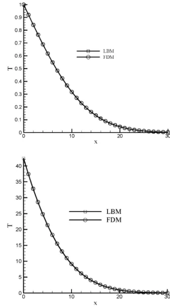
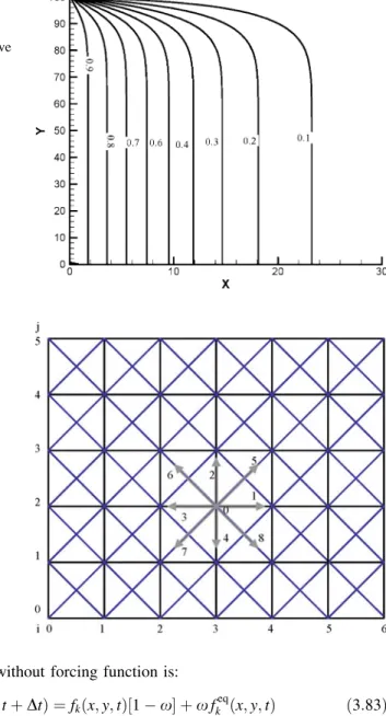
Figure 3.7 shows a comparison of results predicted by LBM and FDM for a plate subjected to a constant heat flux at the boundary.
Axi-Symmetric Diffusion
Two-Dimensional Diffusion Equation
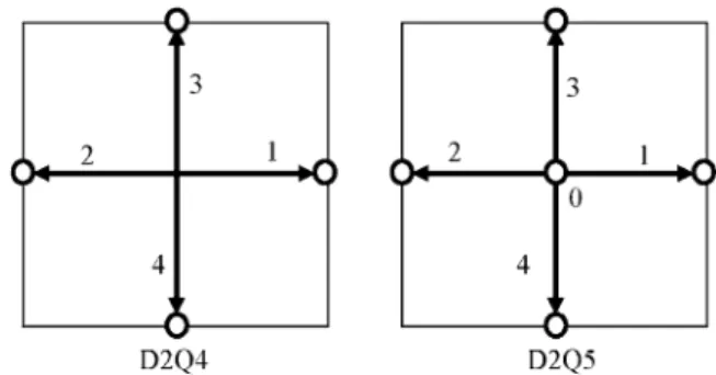
D2Q4
D2Q5
When programming, care must be taken not to overwrite the values, otherwise each step is similar to a 1-D algorithm. Except that every step and algorithm is the same as in D2Q4, of course there is no streaming for particles in the center of the grid (f0).
Boundary Conditions
The Value of the Function is Given at the Boundary
Adiabatic Boundary Conditions, for Instance
Constant Flux Boundary Condition
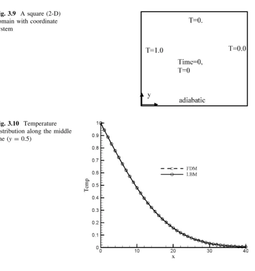
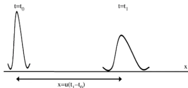
Two-Dimensional Heat Diffusion in a Plate
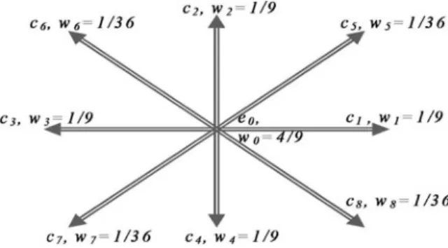
D2Q9
The knowledge gained in solving the diffusion problem using D2Q9 can easily be extended to advection–diffusion and Navier–. For coding simplicity, it is more convenient to use the number of transmission links as shown in Fig.3.12.
Boundary Conditions
The equilibrium function can be calculated using Equation 3.20, fkeqði;jÞ ¼ wðkÞ/ði;jÞin/ði;jÞcan be calculated as,.
Constant Flux Boundary Conditions
Problems
Anisotropic heat diffusion: heat or mass diffusion in wood, crystal, sedimentary rocks and fibers has a preferred direction. The Lattice Boltzmann method will be discussed for solving various advection-diffusion problems for one- and two-dimensional cases.
Advection
Advection–Diffusion Equation
Finite Difference Method
In other words, the accuracy of the solution depends on the ratio of a numerically entered diffusion coefficient to the physical diffusion coefficient (a). Since is positive, the first derivative is approximated as given in the first row of eq 4.4.
The Lattice Boltzmann
Computer code for the 1-D advection-diffusion equation can be found in the appendix for the same problem discussed for the finite difference method. Figure 4.3 compares the results obtained using the finite difference method and the LBM method for the mentioned problem.
Equilibrium Distribution Function
Bicici¼H ð4:19Þ Multiplying both sides of Eq.4.19byxiog from the Chapman–Enskog expansion, the following relation can be obtained. In the following sections, Chapman-Enskog expansion for advection-diffusion problem will be discussed in detail.
Chapman–Enskog Expansion
Two-Dimensional Advection–Diffusion Problems
The top boundary of the domain is kept at zero temperature, while the bottom and vertical right boundaries are assumed to be adiabatic.
Two-Dimensional Lattice Boltzmann Method
D2Q4
The flow and collision processes are similar to what was described in the previous chapter, chap. The computer code (see Appendix) is clear and it is not necessary to elaborate more on the flow and collision processes evaluations, because it is similar to the procedure described in ch.
D2Q9
Note that the scale of the dimension of the problem can be non-dimensionalized or scaled after the calculation. For example, the height and length of the domain can be divided to the total height of the domain, velocity field can be divided to the inlet velocity, and so on.
Problems
Combustion in Porous Layer
The source term S has a value only at the location of heat release and zero at other locations. On entry, x=0; for simplicity, let's assume that Tg=Ts=Tin and at the output x=L; assume that the temperature gradient is zero.
Cooling a Heated Plate
Coupled Equations with Source Term
We will discuss the Lattice Boltzmann Method (LBM) for solving various isothermal two-dimensional fluid flow problems.
Navier–Stokes Equation
Various techniques are available to solve NS equations, such as finite difference, finite volume, finite element, etc. In fact, the major time required to solve NS is spent on solving the Laplace equation.
Lattice Boltzmann
The BGK Approximation
The corresponding Reynolds number can be calculated as Re¼UL=m:U and Lare characteristic velocity and length scale for the given flow. For a given Reynolds number and kinematic viscosity, if the calculated velocity is large, the grid number should be increased.
Boundary Conditions
- Bounce Back
- Boundary Condition with Known Velocity
- Equilibrium and Non-Equilibrium
- Open Boundary Condition
- Periodic Boundary Condition
- Symmetry Condition
Therefore, we need to determine appropriate equations for computing those distribution functions at the boundaries for a given boundary condition. For example, if the pressure is given at the outlet, the following equation can be used to specify the missing distribution functions.
Computer Coding
Examples
Lid Driven Cavity
The simulation results are shown in Figures 5.10 and 5.11 for the flow and velocity at different sections along the cavity, which compare well with the FVM results.
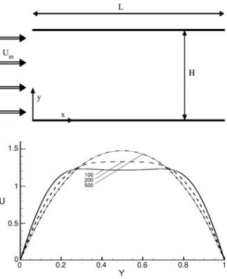
Developing Flow in a Two-Dimensional Channel
This is necessary because at the expiration we assume that the y-component velocity (v) must be zero.
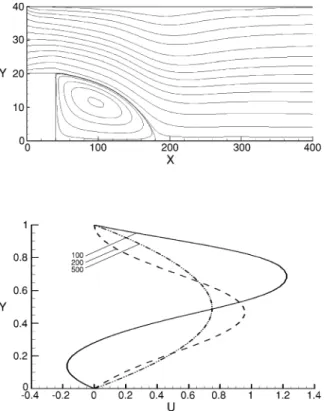
Flow over Obstacles
In the next section, two problems are worked out, namely flow over a backward-facing step and flow over some fixed obstacles embedded in the flow. In the next chapter the non-isothermal problems (forced and natural convection) are discussed.
Vorticity and Stream Function Approach
Hexagonal Grid
Problems
In this chapter, two types of non-isothermal flows, namely forced and natural convection, will be discussed. In forced convection, the energy equation can be solved after the flow field is obtained, i.e., the momentum equation is not coupled to the energy equation.
Naiver–Stokes and Energy Equations
For natural convection (with Bosensque approximations), the governing parameters are Grashof (Gr) or Rayleigh number (Ra), Pr and geometric aspect ratio. For more details on the physics and mathematical modeling of convection, textbooks on heat transfer should be consulted.
Forced Convection, D2Q9–D2Q9
The main driving parameters for forced convection are the Reynolds (Re) and Prandtl (Pr) numbers and the aspect ratio.
Heated Lid-Driven Cavity
Forced Convection Through a Heated Channel
Conjugate Heat Transfer
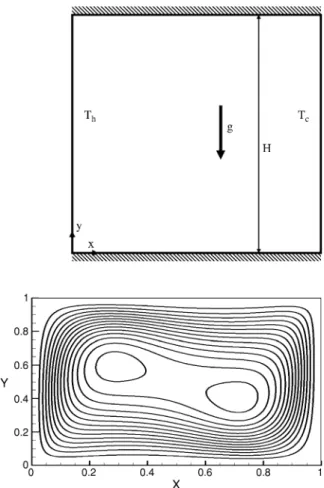
Natural Convection
Example: Natural Convection in a Differentially
The streamlines show perfect oblique symmetry, which is one of the criteria for natural convection in a differentially heated cavity. For higher Ra, more grids were required because the boundary layer becomes thinner as the Rayleigh number increases.
Flow and Heat Transfer in Porous Media
In LBM it must be used in grid units ie. Da¼K=N2; where N is the number of grids in the direction of the characteristic length. There is a claim that multi-relaxation schemes offer a higher stability and accuracy than the single-relaxation scheme.
Multi-Relaxation Method
Furthermore, the entire procedure is the same as for the single relaxation method (SRM).
Problem
Two-Relaxation-Time
Application of the lattice Boltzmann method to the solution of the energy equation of a 2-D transient conduction-radiation problem. Lattice Boltzmann equation for natural convection in a two-dimensional cavity with a partially heated wall.