MONETARY POLICY RULES IN MALAYSIA, SINGAPORE AND THAILAND
Chai-Thing Tan* and Azali Mohamed**
*Corresponding author. Faculty of Business and Finance, Universiti Tunku Abdul Rahman, Malaysia.
Email: [email protected]
**Faculty of Economics and Management, Universiti Putra Malaysia, Selangor D. E., Malaysia.
Email: [email protected]
This paper investigates whether monetary policies in Malaysia, Thailand and Singapore are best represented by either the Taylor rule or the augmented Taylor rule. It finds that the augmented Taylor rule, which incorporates the exchange rate and government spending, best represents monetary policies in these countries. The results show that past inflation and the output gap play a role in the monetary policy reaction function in Malaysia and Thailand. The results further show a strong preference towards interest rate smoothing, government spending, and the exchange rate by the central banks.
Article history:
Received : July 26, 2019 Revised : November 14, 2019 Accepted : August 24, 2020 Available online : December 31, 2020 https://doi.org/10.21098/bemp.v23i4.1112
Keywords: Monetary policy rules; Fiscal policy rules; Monetary and fiscal policy interactions.
JEL Classifications: E52; E58; E62; E63.
ABSTRACT
I. INTRODUCTION
This paper investigates whether monetary policies in Malaysia, Thailand and Singapore are best represented by either the Taylor rule or the augmented Taylor rule. This allows the paper to examine the effectiveness of the central bank’s reaction function in influencing the exchange rate and government spending in these countries over the period of 1980:Q1 to 2017:Q1. To achieve this objective, the study estimates seven different monetary policy reaction functions by oordinary least squares (OLS) and generalized method of moments (GMM).
The central bank of Malaysia (or Bank Negara Malaysia (BNM)) followed a monetary aggregate targeting strategy prior to the mid-1990s to maintain price stability and supportive of economic growth (Said and Ismail, 2008). The BNM changed its monetary policy strategy from monetary aggregate targeting to interest rate targeting in November 1995, mainly due to the instability of the monetary aggregates (Karim and Karim, 2014). The 3-month interbank rate was used as the operational policy target, while the exchange rate regime was free floating within some unannounced band, which is known as a managed float system by the International Monetary Fund (IMF) (Ilzetzki, Reinhart & Rogoff, 2017). In contrast to the BNM, the Monetary Authority of Singapore (MAS) has traditionally used the exchange rate as a policy instrument (Monetary Authority of Singapore, 2001). Singapore dollar is managed against a basket of currencies of its major trading partner. Thus, the MAS designs its monetary policy by following an inflation-targeting exchange rate, rather than by conventional money supply or interest rate targeting, with the primary concern being to promote price stability.
The Bank of Thailand (BoT) pegged the Thai baht to the US dollar from March 8, 1978 to July 1997, changed to freely floating from July 1997 to January 1998, and to manage floating from January 1998 to September 1999 (Ilzetzki, Reinhart &
Rogoff, 2017). The BoT altered its monetary policy rule to monetary-base targeting to achieve its macroeconomic objective of price stability. The BoT changed its monetary policy strategy from monetary-base targeting to inflation targeting since May 2000 (Ilzetzki et al., 2017). These three countries were chosen because they are small open economies with historically low and stable inflation rates—the average inflation rate was 2.96%, 1.94% and 3.62% in Malaysia, Singapore and Thailand, respectively ( see Table 1).
Table 1.
Summary Statistics
This table presents the mean and standard deviation of the variables over the period 1980:Q1 to 2017:Q1 for Malaysia, Singapore and Thailand. The variables are yg = Output gap, π = annualised quarterly inflation rate, i = money market rate, f= government spending, s = nominal exchange rate (domestic currency per US dollar) and ds = first difference of exchange rate, respectively.
Variable Malaysia Singapore Thailand
Mean Standard
Deviation Mean Standard
Deviation Mean Standard Deviation
yg 5.39E-11 4.42 5.5E-11 4.17 3.71E-11 3.17
π 2.96 3.09 1.94 2.86 3.62 4.54
i 4.60 2.12 3.31 3.00 6.80 5.39
f 25847.81 22076.36 6560.62 4722.56 247.50 209.46
s 3.09 0.62 1.69 0.30 31.04 6.91
ds 0.47 4.03 -0.29 2.75 0.35 5.04
The monetary policy reaction function explains how the monetary authority accommodates economic growth or ensures inflation stability by adjusting its policy rule. This simple policy rule, which was developed by Taylor (1993), showed that the United State Federal Reserve Bank could raise the Federal funds rate in the case that (i) the inflation rate is more than two per cent above the implicit target or (ii) the Real Gross Domestic Product (RGDP) is greater than the potential GDP.
This rule has described well the actual direction of the Federal funds rate between the period of 1987 and 1992 (Taylor, 1993). Some have criticised the Taylor rule as being too simplistic because it only considers two variables, namely inflation and the output gap, without taking into consideration other important information needed to conduct monetary policy (Ball, 1999; Moura & De Carvalho, 2010, to name few).
Taylor rule was then rapidly extended and refined into different policy rules, collectively known as Taylor-type rules (Beju & Ciupac-Ulici, 2015). Although, central banks do not explicitly follow an instrument rule, studies have found that Taylor-type rules do have an influence on policy and it could be argued that central banks implicitly follow them (Sánchez-Fung, 2005; Paez-Farrell, 2007). The reaction function of monetary policy can provide guidance to the central banks on setting the interest rate during changing economic conditions while keeping the price level and the economy stable. Taylor rule has become a popular tool for examining the behaviour of central banks, as it provides a straightforward method to estimate the stance of monetary policy.
One of the drawbacks of the simple Taylor rule is that it ignores the characteristics of an open economy. By extending the model to the open economy, the behaviour of the exchange rate becomes an important issue (Senay, 2008).
Few studies showed that the Taylor rule would perform better if it included the exchange rate (Ball, 1999; Moura & De Carvalho, 2010). However, this argument was challenged by Taylor (2001), Chang (2005), Edwards (2007) and Mishkin (2007). So far, empirical evidence on Taylor-type rules has shown overall mixed results (Lubik & Schorfheide, 2007; Garcia et al., 2011; Peiris et al., 2016). Hence, the best model to describe the interest rate is still not clear.
The fiscal theory of price level has explained the impact of fiscal policy on inflation (see Woodford, 2001). As discussed by Davig and Leeper (2011) and Sims (2011), the ultimate impact of fiscal policies on the economy depends on the manner of the interaction between monetary and fiscal policies. Furthermore, the incidence of financial crises has highlighted the importance of policy interaction.
The importance of the interaction of the policies has raised another interesting question: is it necessary for central banks to take into consideration fiscal variables when designing monetary policy?1 Nonetheless, as aforementioned, the literature in this area of research has neglected the role of fiscal policy (Malik, 2013). The behaviour of the exchange rate (Senay, 2008) and decisions made by the fiscal authorities can influence the impact of monetary policy (Davig & Leeper, 2011;
Sims, 2011). Yet, we know little, if any, on the effects of exchange rate and fiscal policies on monetary policy. This study fills this void.
1 See Croushore & Van Norden (2018), and Kitano & Takaku (2016).
The study makes two contributions to the literature. Firstly, it examines the variant of the Taylor rule specification that best describes the behaviour of central banks in Malaysia, Singapore and Thailand during the period of 1980:Q1 to 2017:Q1.
It does this by estimating seven different monetary policy reaction functions using OLS and GMM approaches. Given the importance of the monetary policy reaction functions in macroeconomic modelling, this study is useful because it provides a transparent description of the monetary policy in use in each of the three countries.
Gerlach and Schnabel (2000) suggested that using a rule that is known to the public may help to reduce uncertainty regarding future monetary policy and to avoid instability of the macroeconomic environment. This type of framework has been implemented in advanced economies (see Taylor, 1993; Jondeau & Le Bihan, 2002;
Paez-Farrell, 2007). However, little work has been carried out for emerging and small open economies like Malaysia, Singapore and Thailand. This study adds to the literature by filling this empirical gap and by shedding more light on the monetary policy reaction functions in these three countries.
Secondly, most previous studies have applied and developed the Taylor rule to examine the behaviour of central banks (see Taylor, 1993; Clarida, Galı & Gertle, 1998; Judd & Rudebusch, 1998, among others). Some such as Clarida et al. (2000) focused on amending the rule to include interest rate smoothing, and others such as Ball (1999) noted that the Taylor rule performs better by including exchange rate. There have been very few empirical analyses on monetary policy rules that consider fiscal policy (Kumhof, Nunes, & Yakadina, 2010; Saghir & Malik, 2017).
Kumhof et al. (2010) noted that central banks could better respond to inflation by including the fiscal deficit in their information set. Thus, this paper incorporates the information on government spending in the Taylor rule to enhance the central bank’s reaction function.
The results show that there is a strong preference towards interest rate smoothing, government spending and the exchange rate by the central banks in Malaysia, Singapore and Thailand. More importantly, we find evidence that exchange rate and fiscal policy are very important in explaining the interest rate.
The remaining of this paper is organised as follows. Section II reviews the literature, while Section III describes the model and methodology. Section IV presents the results. Section V concludes.
II. LITERATURE REVIEW
The creation of the Taylor rule has led to an increasing number of studies focusing on central bank rule models and their behaviour (Clarida et al., 1998; Aklan &
Nargelecekenler, 2008). By using quarterly data, Judd and Rudebusch (1998) estimated a simple model of the Federal Reserve’s monetary reaction functions based on the Taylor rule and found that the Taylor rule framework fitted well with the US monetary policy during the period from 1970 to 1997. Seyfried and Bremmer (2001) extended Judd and Rudebusch’s (1998) study by comparing the inclusion of different proxies representing inflation and reached the same conclusion, that the Taylor rules are an effective way to design monetary policy.
From a theoretical point of view, the simple Taylor rule could give a good description of the behaviour of the central banks. However, there are widely held
beliefs that augmented Taylor rules are better fitted than the simple one (Ball, 1999; Moura & De Carvalho, 2010). Several have paid attention to the Taylor rule specification. The research on Taylor-type rules can be distinguished into two strands: (i) the studies dealing with the empirical estimation of the monetary policy reaction function (Taylor, 1993; Clarida et al. 1998, 2000; Haryono, Nugroho,
& Pratomo, 2000); and (ii) those dealing with the determination of an optional monetary policy to achieve the ultimate policy objectives (Jondeau & Le Bihan, 2002; Peersman & Smets, 1999; Svensson, 1999; Juhro, 2008).
Some prior studies have highlighted that the process of a central bank adjusting its policy rate to reach its targeted level is an incremental approach (Clarida et al., 2000). It has been argued that current decisions made by central banks depend on the level of the interest rate in the previous period, assuming that the central bank has full control over the interest rate, and thus leading to the introduction of the idea of interest rate smoothing (Clarida et al., 2000). However, Rudebusch (2002) argued that the inclusion of a lagged interest rate in the Taylor rule owed to the omitted variable problem instead of the smoothing behaviour. However, this argument was challenged by Castelnuovo (2003). Besides that, Gerdesmeier and Roffia (2004) also stated that any smoothing behaviour could be captured by the lagged interest rate when studying interest rate inertia.
In order to investigate the optimal monetary policy required to achieve price stability and full employment, Svensson (1999) argued that simple backwards- looking inflation targeting was the optimal reaction function for monetary authorities. In contrast, Jondeau and Le Bihan (2002) found that forward-looking inflation targeting applied in Germany was optimal because it led to stable inflation and an increase in output. Likewise, Peersman and Smets (1999) revealed that the performance of an optimised Taylor rule was better than the unconstrained optimal feedback rule.
Some researchers have studied the performance of forward-looking, rather than backwards-looking policy. For instance, Clarida et al. (1998) generalised the baseline Taylor (1993) rule by incorporating forward-looking behavior and found that the forward-looking behaviour best characterizes interest rate setting in developed countries, in addition to observing that a policy of fixing the exchange rate might be inferior to an inflation targeting policy. Their findings were supported by Qin and Enders (2008), who found that a forward-looking policy offers a superior fit for developed countries. Furthermore, by estimating the contribution of monetary policy to macroeconomic stability in the US, Clarida et al. (2000) discovered that the interest rate rule was consistent with the Taylor principle after the year 1979 and that their results explained the reason for inflation stability in the US during the early 1980s.
The monetary policy rules proposed by Taylor (1993) are based on the assumption that economies are closed. However, by extending the model to the open economy, the behaviour of the exchange rate becomes an important issue (Esanov et al., 2005; Kharie, 2006; Senay, 2008). Svensson (2000) outlined three ways in which the exchange rate plays a role in the monetary transmission channel. First of all, the real exchange rate influences the relative prices between domestic and foreign goods, subsequently affecting the domestic aggregate demand channel.
Secondly, the exchange rate is important in the forward-looking behaviour and
expectation role in monetary policy. Lastly, foreign disturbances, such as foreign inflation, foreign interest rate changes and investor’s foreign-exchange risk premia are transmitted through the exchange rate.
Ball (1999) claimed that the Taylor rule would perform better if it included the exchange rate and showed that countries tended to increase their interest rates to deal with real currency depreciation. Similarly, Moura and De Carvalho (2010) demonstrated that Taylor rules with exchange rates produced a superior predictability results in seven Latin American emerging economies as compared with the simple Taylor rule. The exchange rate transmission effect has been validated by Hsing (2004) and Hsing and Lee (2004), who studied the monetary reaction function of the Bank of Canada and the Bank of Korea. However, the argument for the inclusion of the exchange rate in the Taylor rule has been challenged by Taylor (2001). He claimed that the inclusion of the exchange rate worsened the objective of the stabilisation policies because the exchange rate plays no role in a forward- looking reaction as there is an indirect effect of the exchange rate in interest rates through inflation. This opinion has been agreed upon by Chang (2005), Edwards (2007) and Mishkin (2007). Moreover, Osawa (2006) uncovered that the central banks in the East Asian inflation targeting countries2 did not react to the exchange rate. A similar result was found by Sek (2009)3 who extended Osawa’s (2006) study by including a structural break.
Over the years, fiscal policy has received considerable attention (Kneller et al., 1999; Perotti, 1999; Tanzi & Schuknecht, 2003; Alexiou, 2009; Alshahrani &
Alsadiq, 2014) due to its relevance and impact on other policies, such as monetary policy. A tight fiscal space4 not only restricts the use of fiscal policy instruments but also constrains the use of monetary policy instruments (Abdel-Haleim, 2016).
For instance, the financing of budget deficits through the issuance of bonds may put upward pressure on the domestic cost of credit and cause the central bank to ease this pressure through monetary policy tools, ultimately pushing up the inflation rate. In short, a lack of fiscal space causes fiscal instruments to lose their effectiveness and makes the coordination between monetary and fiscal policies difficult. In addition, central banks follow fiscal policy stabilisation to achieve price stability (Abdel-Haleim, 2016).
Recent studies have shown that it is necessary for central banks to take into consideration fiscal variables when designing monetary policy (Kitano &
Takaku, 2016; Croushore & Van Norden, 2018). By including fiscal solvency and fiscal deficit, central banks could obtain a better ability to respond to inflation aggressively (Kumhof et al., 2010) and determine the interest rate (Saghir & Malik, 2017). In contrast, Hasanov and Omay (2008) discovered that the Turkish monetary authority reacted to budget deficits only during periods of economic expansion.
Meanwhile, Zoli (2005) revealed that the fiscal stance of emerging market countries did not influence the conduct of monetary policy.
2 Osawa’s (2006) study focused on Korea, Thailand and the Philippines.
3 Sek (2009) found that there was a weak reaction of the policy function towards exchange rate movements pre- and post- financial crisis of 1997, in two out of the three countries.
4 Fiscal space is defined as “the availability of budgetary room that allows a government to provide resources for a desired purpose without prejudice to the sustainability of a government’s financial position” (Heller, 2005).
To the best of our knowledge, only a few published empirical studies, such as Umezaki (2007) Ramayandi (2007) and Hsing (2009), have estimated the central bank’s monetary reaction functions for Malaysia, Thailand and Singapore.
Umezaki (2007) examined the monetary policy reaction function of the BNM using monthly data and found that the BNM’s behaviour was affected by changes in the exchange rate regime and the degree of capital mobility. Meanwhile, Ramayandi (2007) estimated the monetary policy reaction function in five ASEAN countries, including the three countries in our study. He used the Henderson-Mckibbon- Taylor interest rate and a shorter sample period of 1989Q1 to 2014Q4. Hsing (2009) found that the central banks of Indonesia, Malaysia, the Philippines and Thailand reacted positively to inflation and the output gap and that the central banks in Indonesia and Thailand reacted more aggressively to inflation when compared with other countries.
The monetary policy reaction function in our paper is largely similar to those specified in Umezaki (2007), Ramayandi (2007) and Hsing (2009), but differs from others because it incorporates new features. For example, we cover a longer sample period (i.e. from 1980Q1 to 2017Q1) and augment the Taylor rule to capture the role of exchange rate and fiscal policy. This longer period covers different stages of economic development experienced by the countries, and hence provides a better view of the central bank’s reaction function under different economic circumstances. Further, recent studies have shown the importance of fiscal policy (Kitano & Takaku, 2016; Croushore & Van Norden, 2018). However, no consensus was reached regarding whether the central bank should target fiscal policy variables. Thus, this this paper provides evidence relating to the roles of the exchange rate and government spending in the central bank’s reaction function.
III. METHODOLOGY A. Taylor Rule Specification
To establish the best Taylor rule specification, the study estimated seven different models. Equation (1) is the simplest (contemporaneous) Taylor rule with interest rate smoothing.
where θπ shows the central bank’s stance on inflation. If the priority of the central bank is to fight inflation, then θπ >1. Similarly, if 0< θπ <1, then the central bank reacts by increasing the interest rate in order to reduce inflation. This condition is only able to accommodate inflation as an increase in the interest rate is not sufficient to cause the real interest rate to reduce. βy shows the central bank’s stance on the output gap. If βy > 0, then the interest rate moves to stabilise output. 0≤ ρ ≤1 is a smoothing coefficient, which captures the persistence of the market interest rate.
It indicates how strictly the central bank follows the policy rule, thus larger values of ρ indicate a slower adjustment speed. The error term ε is an exogenous random shock to the interest rate.
Equations (2) and (3) are the forward- and backward-looking Taylor rules, respectively. Equation (2) replaces inflation, πt, in Equation (1) with the expected (1)
inflation rate for the next quarter, (Kozicki, 1999; Clarida et al., 1998) and the output gap, , with the expected output gap for next quarter ahead, .
where is a linear
combination of the forecast errors of inflation and the output gap.
Some studies have shown that a forward-looking rule has a superior fit for developed countries (Qin and Enders, 2008), but due to imperfect credibility of central banks, backward-looking inflation may affect inflation expectation in emerging economies (Moura and De Carvalho, 2010). Further, the values of future inflation and output gap are unknown, thus they are replaced with the values of lagged π and yg (Kozicki, 1999). Equation (3) is the backward-looking Taylor rule, whereby the policy reacts to the previous quarter’s inflation and the output gap.
(2)
where πt-1and ygt-1 denote, respectively, the inflation rate and the output gap for the previous quarter.
Some (Ball, 1999; Moura & De Carvalho, 2010) have criticised the Taylor rule as being too simplistic because it only considers two variables, namely inflation and the output gap, without taking into consideration other important information needed to conduct monetary policy. By assuming that exchange rate stability is one of the objectives of the central bank, the study extended Equation (2) and (3) by including the exchange rate in line with Molodtsova and Papell (2009), and Moura and De Carvalho (2010). This allowed the study to examine how the central bank reacts to the exchange rate besides inflation and the output gap. The following are the forward- and backward-looking Taylor rules with the exchange rate.
(3)
where βs is the coefficient of the exchange rate and st is the exchange rate at period t. The central bank will increase the interest rate to stabilise the currency, if the exchange rate depreciates. Therefore, βs >0 if the exchange rate is quoted as domestic currency per unit of the foreign currency. However, the interest rate will remain relatively low when the exchange rate appreciates. If βs =0, the central bank does not change the interest rate to stabilise the exchange rate.
The most economists have focused on the interaction between monetary and fiscal policies (see Kirsanova, Leith & Wren-Lewis, 2009; Fragetta, & Kirsanova, 2010, Tan, Mohamed, Habibullah & Chin, 2020). However, the Taylor rule does not take into consideration fiscal policy. How does fiscal policy influence the Taylor rule if fiscal policy variables are visibly absent from the central bank’s reaction (4) (5)
function? By extending the Taylor rule to incorporate fiscal policy variables, this study is able to examine the influence of fiscal policy on the Taylor rule. In order to ensure that the intertemporal budget constraint of the government holds, the central bank must accommodate fiscal shocks. The central bank is the only institution able to ensure fiscal solvency in order to stabilise the price level, therefore, it should react to fiscal variables when setting its policy. To examine these issues, the fiscal variables at t, ft are added to Equations (4) and (5) to form Equations (6) and (7). The extended forward- and backward-looking Taylor rules with the fiscal variables are as follows.5
where βf is the coefficient of government spending. A negative sign on βf implies that when fiscal policy is expansionary (increase in government spending or budget deficit), the central bank will expand monetary policy (reduce the interest rate). This is in line with Sargent and Wallance (1981), who found that fiscal expansions eventually trigger an expansionary monetary policy. βf <0 implies that borrowing from the central bank weakens the monetary policy stance (Saghir and Malik, 2017). On the other hand, βf >0 implies that government spending and interest rate change in the different direction, which is an indication that monetary and fiscal policies move in conflicting directions. This also implies that the effect of borrowing from commercial banks outweighs the effect of borrowing from the central bank (Saghir and Malik, 2017). βf =0 indicates that government spending does not directly affect the conduct of the central bank.
In our application, given that Singapore manages its monetary policy using the Singapore dollar exchange rate and uses exchange rate targeting as its monetary policy, some further attention is required in the case of Singapore. In order to compare Singapore with the other countries, this study followed (Ramayandi, 2007) and used the interest rate as an instrument for approximating monetary policy in Singapore by exploiting the uncovered interest rate parity theory.
B. Generalized Method of Moment (GMM)
This study estimated the seven specifications (Equations (1) to (7)) using quarterly data from 1980Q1 to 2017Q1. Equation (1) is the standard Taylor rule, which we estimated by the OLS method with the Newey-West standard errors. Meanwhile, the other models were estimated using the GMM estimation method. As Equations (2) to (7) included inflation and the output gap, the estimates would be biased if estimated by OLS. This is because OLS does not maintain stability due to nonlinearity in the model. Therefore, the GMM estimator of Hansen (1982) was the most appropriate estimator for estimating these equations.
5 Following Kumhof et al., (2010), we modeled fiscal variables using the government spending and assumed that the tax rate remained constant.
(6) (7)
In addition, there were other reasons for using the GMM method to estimate the Taylor rules. Firstly, the GMM approach provided a simple way to test the validity of the specifications and did not involve a normality assumption. Secondly, by using the weighting matrix, the GMM estimator made the estimates robust to both heteroscedasticity and autocorrelation. Thirdly, GMM estimators do not suffer from simultaneity bias. Finally, the GMM approach has been used in other empirical tests of the Taylor rules, such as Yazgan and Yilmazkuday (2007), Paez- Farrell (2007) and Aklan and Nargelecekenler (2008), to name a few.
The GMM estimation method depends on a set of instruments, Zt. To run the GMM estimation of the Taylor rule, a set of instrument variables was chosen. This paper followed Paez-Farrell (2007) and used four lags of each of the explanatory variables as the instrument variables. The list of instruments is a constant term and the first 4 lags of the interest rate, inflation, the output gap, the exchange rate and government spending. Last, to test the validity of the instruments, the study applied the Hansen (1982) J-test. The null hypothesis of the J-test is that the model is valid. Thus, failure to reject the null hypothesis indicated that the instruments used were appropriate.
C. Data
The sample period of this study is from 1980: Q1 to 2017: Q1, leading to a total of 149 observations for the three countries, namely Malaysia, Singapore and Thailand. The money market rate (it) is used as a proxy for the monetary policy instrument. The annualised quarterly inflation rate (πt) is the difference of the logarithm of the consumer price index (CPI) with base year 2010=100 (i.e. πt≡400 (lnCPIt - lnCPIt-1)). Output gap (ytg) is the change between the logarithm of the real RGDP and the logarithm of the potential GDP, i.e. ytg ≡ yt - yt*, which is the Hodrick- Prescott (HP) filtered RGDP, where yt =lnRGDPt.6 To calculate potential output using the HP filter, we set the smoothing parameter to λ=1600 because the data is quarterly. The exchange rates were measured using the natural logarithm of the nominal exchange rate (i.e. st = domestic per US dollar). An increase in the nominal exchange rate, st, implies a depreciation in the home currency against the US dollar. Government spending (ft) is used to proxy for the fiscal policy instrument.
Following Agnello and Sousa (2011), the paper used government spending as the fiscal policy instrument instead of the government revenue because data on government spending is available in the three selected countries at quarterly frequency (see also Fragetta and Kirsanova, 2010). The data were extracted from the International Financial Statistics published by the IMF. All the data, excluding the interest rate, were converted into logarithmic form.
6 We used the HP filter because it is the most widely used approach for determining the potential output gap (yt*), especially in studies on the Taylor rule (see e.g. Molodtsova and Papell, 2009;
Papadamou et al., 2018).
IV. EMPIRICAL RESULTS A. Descriptive Statistics
Table 1 presents the mean and standard deviation for inflation, output gap, interest rate, exchange rate and government spending for Malaysia, Singapore and Thailand. The output gap (with values close to zero) was quite similar for all three countries. The inflation in Singapore was the smallest, when compared to Malaysia and Thailand. Thailand recorded a relatively high money market rate as compared to Malaysia and Singapore over the same period. When compared to the money market rate, government spending showed more variability across the countries. The exchange rate was also highest for Thailand (recording an average of 31.04 baht per US dollar) over the period, followed by Malaysia (3.09 Ringgit per US dollar) and Singapore (1.69 Singapore dollar per US dollar), but the Singapore dollar had the least variability over the sample period.
B. Data Analysis
The GMM estimator relies on the stationarity of the data. Therefore, in order to apply the GMM estimator, all the series, including the instrumental variables, must be stationary. Since there is a likelihood that the variables used in this study are non-stationary, they were tested using the Augmented Dickey-Fuller (ADF) and the Phillips–Perron (PP) tests to determine whether they are stationarity. The null hypotheses of both tests are that the variable have a unit root. Thus, if the t-statistic under the null is more negative than the critical value, then we rejected the null hypotheses and concluded that the variables were stationary.
Table 2.
Unit Root Test Results
This table presents unit root test results for Malaysia, Singapore and Thailand. The variables are yg = Output gap, π= annualised quarterly inflation rate, i = money market rate, f = government spending, s = nominal exchange rate (domestic currency per US dollar) and ds = first difference of exchange rate, respectively. The null hypothesis of the ADF and PP tests is that the variable contains a unit root. ***, **, and * denote significance at 1%, 5%, and 10%, respectively.
Variable Malaysia Singapore Thailand
ADF PP ADF PP ADF PP
Panel A: Level
yg -4.9(12)*** -5.3(7)*** -5.3(8)*** -5.3(8)*** -4.6(12)*** -7.3(9)***
π -9.6(0)*** -9.7(5)*** -4.2(7)*** -7.2(4)*** -8.8(0)*** -8.7(7)***
i -3.7(6)* -3.6(2)** -3.2(11)* -3.4(5)* -4.4(3)*** -3.6(2)**
f -3.3(8)* -14.2(11)*** -3.2(13)* -11.9(11)*** -1.6(9) -7.9(10)***
s -2.3(1) -2.1(1) -2.4(7) -1.77(3) -1.9(0) -1.9(5)
ds -10.9(0)*** -10.9(5)*** -12.8(0)*** -12.8(2)*** -11.8(0)*** -11.8(8)***
Panel B: First Difference
yg -5.5(13)*** -11.9(8)*** -5.8(9)*** -13.8(9)*** -4.1(13)*** -18.2(10)***
π -7.5(6)*** -44.6(28)*** -8.5(0)*** -8.4 (1)*** -8.0(5)*** -17.9(2)***
i -9.6(1)*** -8.8(8)*** -4.6(10)*** -12.8(10)*** -4.8(12)*** -9.9(4)***
f -4.6(10)*** -54.8(14)*** -3.3(11)* -37.7(14)*** -4.6(7)*** -30.2(12)***
s -10.9(0)*** -10.9(5)*** -12.4(0)*** -12.4(2)*** -11.80)*** -11.8(9)***
ds -8(6)*** -78.3(65)*** -9(5)*** -82.8(52)*** -6.5(12)*** -82.1(54)***
From Table 2, we concluded that all the variables were stationary at levels, except for the exchange rate, which we found to be stationary at first difference.
Thus, to run the GMM test, we differenced the exchange rate once to ensure stationarity.
In line with the study’s objective, we compared the seven specifications of the Taylor rule, namely (i) simple, forward and backward reaction (ii) forward and backward reaction to exchange rate movements, and (iii) forward and backward reaction to both exchange rate and government spending movements for Malaysia, Singapore and Thailand.
C. Baseline Model
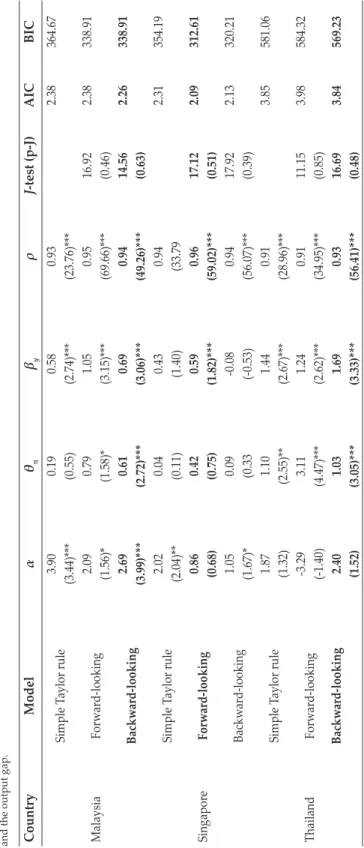
This section reports the estimates of the baseline policy reaction function for the three countries. Table 3 reports the baseline contemporaneous, forward-looking, and backward-looking Taylor rules. The first four columns of Table 3 report the estimates of α, βπ, βy, and ρ with t-statistics in parentheses. The t-statistics are calculated based on heteroscedasticity and autocorrelation robust Newey-West standard errors. The bolded values show the best baseline models. The standard measures of fit, represented by the Akaike Information Criteria (AIC) and Schwarz Bayesian Information Criterion (BIC) are report in the sixth and seventh columns of Table 3. The models were able to track the interest rate movements well, as shown by the relatively low AIC and BIC results. Moreover, the Hansen J-test results also validated the instrument variables. As shown in Table 3, the best-fitted monetary policy response functions in Malaysia and Thailand were backwards- looking, while for Singapore it was forward-looking. In other words, in Malaysia and Thailand, the best estimate obtained was one-quarter lag inflation, which meant that the monetary policy of these countries reacted to inflation a fourth- quarter behind. Conversely, the Singapore model was best-fitted one-quarter- ahead of inflation.
In addition, a few interesting messages have been delivered from the results.
Three countries were found to have a high degree of interest rate smoothing because the coefficients of the lagged interest rate were recorded at between 0.93 and 0.96. Besides that, the estimated values of θπ for all three countries studied had the expected positive sign and were significant for both Malaysia and Thailand (but not for Singapore). In Malaysia, the central bank responded positively by 61% to the inflation rate; meanwhile, the interest rate moved to accommodate inflation in Thailand. This result implied that the monetary authorities of these two countries should adopt a countercyclical policy.
On the other hand, the output gap for all the countries were statistically significant and have positive coefficients, consistent with the theoretical expectation that the central banks would increase the interest rate to stabilise economic growth. Among the three countries, Thailand was the most sensitive to output gap movements because it has the highest output gap coefficient, which was 1.69, compared to 0.6 and 0.59 for Malaysia and Singapore, respectively. Overall, the specifications of the Taylor rule provided an appropriate benchmark for further analysis.
Table 3. Estimated Baseline Taylor Rule (1980: Q1-2017: Q1) This table reports the baseline model estimates for each country. The bolded estimates show the best baseline models. The values in the parentheses are t-statistics. ***, **, and * denote significance at 1%, 5%, and 10%, respectively. J-test and p-J denote, respectively, Hansen J-statistic and its p-value. The backward- (forward-) looking model is one lag (lead) for inflation and the output gap. CountryModelαθπβyρJ-test (p-J)AICBIC Malaysia
Simple Taylor rule3.900.190.580.932.38364.67 (3.44)***(0.55)(2.74)***(23.76)*** Forward-looking2.090.791.050.9516.922.38338.91 (1.56)*(1.58)*(3.15)***(69.66)***(0.46) Backward-looking2.690.610.690.9414.562.26338.91 (3.99)***(2.72)***(3.06)***(49.26)***(0.63) Singapore
Simple Taylor rule2.020.040.430.942.31354.19 (2.04)**(0.11)(1.40)(33.79 Forward-looking0.860.420.590.9617.122.09312.61 (0.68)(0.75)(1.82)***(59.02)***(0.51) Backward-looking1.050.09-0.080.9417.922.13320.21 (1.67)*(0.33(-0.53)(56.07)***(0.39) Thailand Simple Taylor rule1.871.101.440.913.85581.06 (1.32)(2.55)**(2.67)***(28.96)*** Forward-looking-3.293.111.240.9111.153.98584.32 (-1.40)(4.47)***(2.62)***(34.95)***(0.85) Backward-looking2.401.031.690.9316.693.84569.23 (1.52)(3.05)***(3.33)***(56.41)***(0.48)
D. Augmented Taylor Rule for the Exchange Rate Table 4. Estimated Taylor Rule with the Exchange Rate (1980: Q1- 2017: Q1) This table reports estimates of the augmented Taylor rule model with exchange rate for each country. The bolded estimates show the best augmented Taylor rule with exchange rate. ***, **, and * denote significance at 1%, 5%, and 10%, respectively. J-test and p-J denote, respectively, the Hansen J-statistic and its p-value. The backward- (forward-) looking model is one lag (lead) for inflation and the output gap. CountryModelαθπβyβsρJ-test (p-J)AICBIC MalaysiaForward-looking1.211.140.521.730.9113.602.94437.57 (0.79)(1.94)*(1.68)*(2.05)***(26.53)***(0.63) Backward-looking2.990.430.381.180.8912.082.23337.86 (5.35)***(2.62)***(2.34)***(2.09)**(24.41)***0.74 SingaporeForward-looking-2.910.090.300.100.8614.472.002303.14 (-4.13)***(0.61)(2.59)**(8.80)***(35.67)***0.56 Backward-looking-3.260.160.070.110.8614.172.08316.37 (-4.38)***(1.25)(0.98)(6.45)***(37.00)***(0.59) ThailandForward-looking-2.752.560.800.700.9013.173.92578.95 (-1.55)(5.35)***(2.55)**(1.79)*(34.53)***(0.66) Backward-looking1.550.940.861.210.9314.683.79564.93 (1.26)(3.17)***(2.40)**(2.32)**(45.86)***(0.55)
From Table 4, the best augmented Taylor rule model for the exchange rate in Malaysia and Thailand was backward-looking, meanwhile, for Singapore, it was forward-looking; these results were consistent with the baseline model. Again, all the countries exhibited a high degree of interest rate smoothing. Inflation has a significant positive coefficient in all the countries, except for Singapore— inflation was not the core focus of Singapore’s monetary policy. Besides, the response of the interest rate to inflation was stronger in Thailand when compared to Malaysia.
Similar to the baseline model, the central bank responded positively to the output gap in the three countries, the response being strongest in Thailand, followed by Malaysia and then Singapore. Except for Singapore, the response of the inflation rate to interest rate in Malaysia and Thailand was greater than the response of the output gap to interest rate, meaning that the main task of the central banks was to achieve price stability by adequately controlling the inflation rate.
Looking into the effect of the exchange rate, the positive coefficient recorded by the three countries indicated that local currency depreciation will lead to monetary tightening through increases in the interest rate. Besides that, the results implied that the exchange rate was one of the important components when determining the interest rate. This result supported the findings of Peiris et al. (2016), who pointed out that the role of the exchange rate in monetary policy in emerging countries was greater than in advanced countries because of the stronger exchange rate pass- through to inflation in less developed financial markets. Overall, the augmented Taylor rule estimates were similar to those of Caporale et al. (2018), Filosa (2001) and Monagaran and Sek (2016).
D. Augmented Taylor Rule for the Exchange Rate and Government Spending
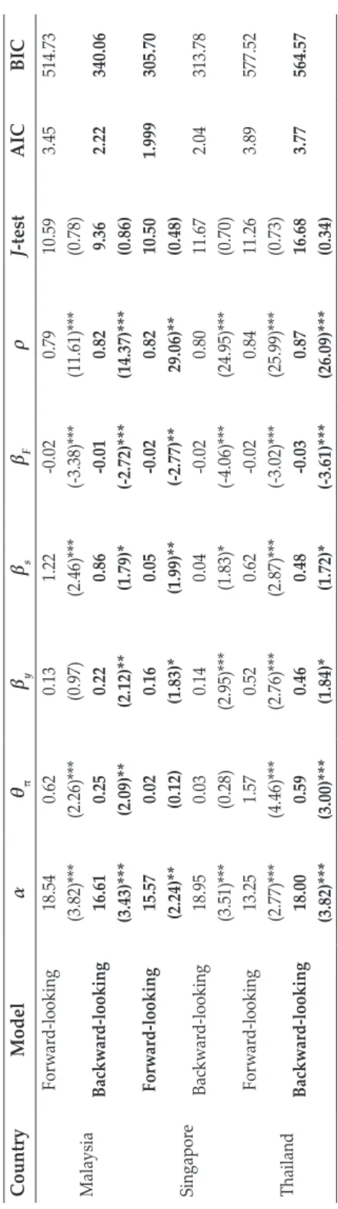
Finally, Table 5 answers the last question regarding whether government spending influences the interest rate, independent of its impact on the output gap and inflation. The estimates on the monetary policy response and interest rate smoothing behaviour were consistent in the previous two sections, indicating the robustness of the models. The estimate of the interest rate smoothing behaviour was consistent with Clarida et al. (2000) and Brüggemann and Thornton (2003).
The estimates in Table 5 suggested that the coefficients of government spending for all the countries were negative. The statistical significance of the coefficients showed that government spending influenced the decisions of the central banks, whereby the central banks eased monetary policy when the government expanded its spending. This finding was consistent with Croushore and Norden (2018) and Saghir and Malik (2017) who found that a higher budget deficit led to an interest rate cut. As a result, the central banks should consider fiscal policy variables in designing monetary policy because they are the only institution that can ensure fiscal solvency.
Table 5. Estimated Taylor Rule with the Exchange Rate and Government Spending from 1980: Q1-2017: Q1 This table reports estimates of the augmented Taylor rule model with exchange rate and government spending for each country. The bolded estimates show the best augmented Taylor rule models with exchange rate and government spending. ***, **, and * denote significance at 1%, 5%, and 10%, respectively. J-test and p-J denote, respectively, the Hansen J-statistic and its p-value. The backward- (forward-) looking model is one lag (lead) for inflation and the output gap. CountryModelαθπβyβsβFρJ-testAICBIC Malaysia
Forward-looking18.540.620.131.22-0.020.7910.593.45514.73 (3.82)***(2.26)***(0.97)(2.46)***(-3.38)***(11.61)***(0.78) Backward-looking16.610.250.220.86-0.010.829.362.22340.06 (3.43)***(2.09)**(2.12)**(1.79)*(-2.72)***(14.37)***(0.86) Singapore
Forward-looking15.570.020.160.05-0.020.8210.501.999305.70 (2.24)**(0.12)(1.83)*(1.99)**(-2.77)**29.06)**(0.48) Backward-looking18.950.030.140.04-0.020.8011.672.04313.78 (3.51)***(0.28)(2.95)***(1.83)*(-4.06)***(24.95)***(0.70) Thailand Forward-looking13.251.570.520.62-0.020.8411.263.89577.52 (2.77)***(4.46)***(2.76)***(2.87)***(-3.02)***(25.99)***(0.73) Backward-looking18.000.590.460.48-0.030.8716.683.77564.57 (3.82)***(3.00)***(1.84)*(1.72)*(-3.61)***(26.09)***(0.34)
Figure 1.
Trends of the Variables from 1980Q1 to 2017Q1 in Malaysia
This figure shows the trends of the variables used in Malaysia. The variables are MMR = money market rate, INF = inflation rate, YG = Output gap, DLER = first difference of exchange rate, and LG = government spending.
1980 1985 1990 1995 2000 2005 2010 2015
0 2 4 6 8 10
12 MMR
1980 1985 1990 1995 2000 2005 2010 2015
-10 -5 0 5 10 15
20 INF
Figure 1.
Trends of the Variables from 1980Q1 to 2017Q1 in Malaysia (Continued)
1980 1985 1990 1995 2000 2005 2010 2015
-15 -10 -5 0 5 10
15 YG
1980 1985 1990 1995 2000 2005 2010 2015
-10 0 10 20
30 DLER
1980 1985 1990 1995 2000 2005 2010 2015
800 900 1,000 1,100
1,200 LG
Figure 2.
Trends of the Variables from 1980Q1 to 2017Q1 in Singapore
This figure shows the trends of the variables used in Singapore. The variables areMMR = money market rate, INF= inflation rate, YG = Output gap, DLER = first difference of exchange rate, and LG = government spending.
1980 1985 1990 1995 2000 2005 2010 2015
0 4 8 12
16 MMR
1980 1985 1990 1995 2000 2005 2010 2015
-10 -5 0 10
5
15 INF
Figure 2.
Trends of the Variables from 1980Q1 to 2017Q1 in Singapore (Continued)
1980 1985 1990 1995 2000 2005 2010 2015
-15 -10 -5 0 10 5
15 YG
1980 1985 1990 1995 2000 2005 2010 2015
-8 -4 0 8 4
12 DLER
1980 1985 1990 1995 2000 2005 2010 2015
LG
700 750 800 850 900 950 1,000 1,050
Figure 3.
Trends of the Variables from 1980Q1 to 2017Q1 in Thailand
This figure shows the trends of the variables used in Thailand. The variables are MMR = money market rate, INF= inflation rate, YG = Output gap, DLER = first difference of exchange rate, and LG = government spending.
1980 1985 1990 1995 2000 2005 2010 2015
MMR
0 5 10 15 20 25
1980 1985 1990 1995 2000 2005 2010 2015
INF
-20 -10 0 10 20 30
Figure 3.
Trends of the Variables from 1980Q1 to 2017Q1 in Thailand (Continued)
1980 1985 1990 1995 2000 2005 2010 2015
YG
-15 -10 -5 0 5 10
1980 1985 1990 1995 2000 2005 2010 2015
DLER
-30 -20 -10 0 10 20 30 40
1980 1985 1990 1995 2000 2005 2010 2015
LG
300 400 500 600 700
For a better understanding regarding how well the Taylor rules explained the behaviour of the central banks in Malaysia, Singapore and Thailand, this study plotted the actual interest rate and the developments of the fitted interest rate rule (see, Appendix 1-3). Each figure shows three panels: Panel A presents the baseline model; and Panels B and C present the augmented Taylor rule model with or without government spending. By observing each of the panels, a difference is shown between the three sets. Overall, the distance between the predicted interest rate and the actual interest rate is very close throughout the sample. The interest rate implied by the backward-looking rule for Malaysia and Thailand and the forward-looking rule for Singapore fit behaviour of the actual interest rate reasonably well. Nevertheless, the model looks to better fit the data after the Asian financial crisis from 1999: Q1 to 2017: Q1. This was consistent with Cavoli and Rajan (2008). This suggested that the central banks should use the augmented Taylor rule during the post-crisis period.
V. CONCLUSION
Taylor rule provides an easy and a transparent description of the behaviour of central banks. This study showed that the estimated monetary policy reaction functions were well fitted and followed the trend of the actual interest rate over the years. The monetary authorities in Thailand and Malaysia do follow the augmented Taylor rule as the inflation and the output gap coefficients were statistically significant and positive in both countries. However, the estimates did not satisfy the Taylor principle that the coefficient of the inflation rate needed to be more than one, while that of the output-gap must be 0.5.
Besides, by using different specifications, the estimated smoothing coefficient of the monetary policy reaction function was statistically significant at a relatively high value (i.e. between 0.7 and 0.9), which proved the tendency of the central banks to lean towards the past interest rate in Malaysia, Singapore and Thailand.
The size of the estimated smoothing parameter was comparable with other related studies in developing countries and industrialised countries.
The augmented Taylor rule with both the exchange rate and government spending performed better than the ones without the exchange rate and government spending, showing that these two variables played an essential role in determining the interest rates in Malaysia, Singapore and Thailand. Even government spending had an impact on the augmented Taylor rule but the effect was relatively small.7 Besides, the fiscal environment was one of the factors that affected the policy rates in Malaysia, Thailand and Singapore. Thus, if the monetary authorities in these countries want to control prices or stabilise outputs, they will not be successful unless fiscal discipline is maintained. There is a need for policy coordination to affect the target variables in the desired direction.
7 One of the reasons is that fiscal dominance has not been a serious issue, at least during the period of our study, or does not have a conflict between the issue of divergent policy goals (Kuttner, 2002).
REFERENCES
Abdel-Haleim, S.M. (2016). Coordination of Monetary and Fiscal Policies: The Case of Egypt. International Review of Research in Emerging Markets and the Global Economy, 2, 933-954.
Agnello, L., & Sousa, R. M. (2011). Can Fiscal Policy Stimulus Boost Economic Recovery?. Revue économique, 62, 1045-1066.
Aklan, N. A., & Nargelecekenler, M. (2008). Taylor Rule in Practice: Evidence from Turkey. International Advances in Economic Research, 14, 156-166.
Alexiou, C. (2009). Government Spending and Economic Growth: Econometric Evidence from the South Eastern Europe (SEE). Journal of Economic and Social Research, 11, 1-16.
Alshahrani, M. S. A., & Alsadiq, M. A. J. (2014). Economic growth and government spending in Saudi Arabia: An empirical investigation. International Monetary Fund.
Ball, L. (1999). Policy Rules for Open Economies. In: Taylor, J. B., Monetary Policy Rules. Chicago: University of Chicago Press, 127-144.
Beju, D. G., & Ciupac-Ulici, M. L. (2015). Taylor Rule in Emerging Countries.
Romanian case. Procedia Economics and Finance, 32, 1122-1130.
Brüggemann, I., & Thornton, D. L. (2003). Interest Rate Smoothing and the Specification of the Taylor Rule. Fachbereich Wirtschaftswiss. der Freien Univ.
Caporale, G. M., Helmi, M. H., Çatık, A. N., Ali, F. M., & Akdeniz, C. (2018).
Monetary Policy Rules in Emerging Countries: Is There an Augmented Nonlinear Taylor Rule? Economic Modelling, 72, 306-319.
Castelnuovo, E. (2003). Taylor Rules, Omitted Variable, and Interest Rate Smoothing in the US. Economic Letters, 81, 55-59.
Cavoli, T., & Rajan, R. S. (2008). Open Economy Inflation Targeting Arrangements and Monetary Policy Rules: Application to India. Indian Growth and Development Review, 1, 237-251.
Chang, H. S. (2005). Estimating the Monetary Policy Reaction Function for Taiwan:
A VAR model. The International Journal of Applied Economics, 2, 50-61.
Clarida, R., Gali, J., & Gertler M. (2000). Monetary Policy Rules and Macroeconomic Stability: Evidence and Some Theory. The Quarterly Journal of Economics, 65, 147-180.
Clarida, R., Galı, J., & Gertler, M. (1998). Monetary Policy Rules in Practice: Some International Evidence. European Economic Review, 42, 1033-1067.
Croushore, D., & Van Norden, S. (2018). Fiscal Forecasts at the FOMC: Evidence from the Greenbooks. Review of Economics and Statistics, 100, 933-945.
Davig, T., & Leeper, E. M. (2011). Monetary–Fiscal Policy Interactions and Fiscal Stimulus. European Economic Review, 55, 211-227
Edwards, S. (2007). The Relationship Between Exchange Rates and Inflation Targeting Revisited. Central Banking, Analysis, and Economic Policies Book Series, 11, 373-413.
Esanov, A., Merkel, C., & de Souza, L. V. (2017). Monetary Policy Rules for Russia.
Journal of Comparative Economics, 33,484-499.
Filosa, R. (2001). Monetary Policy Rules in Some Mature Emerging Economies. BIS pap, 8, 39–68.