Network Layer:
Delivery, Forwarding, and Routing
This chapter describes the delivery, forwarding, and routing of IP packets to their final destinations. Deliveryrefers to the way a packet is handled by the underlying networks under the control of the network layer. Forwardingrefers to the way a packet is deliv- ered to the next station. Routingrefers to the way routing tables are created to help in forwarding.
Routing protocolsare used to continuously update the routing tables that are con- sulted for forwarding and routing. In this chapter, we also briefly discuss common uni- cast andmulticast routingprotocols.
22.1 DELIVERY
The network layer supervises the handling of the packets by the underlying physical networks.We define this handling as the delivery of a packet.
Direct Versus Indirect Delivery
The delivery of a packet to its final destination is accomplished by using two different methods of delivery, direct and indirect, as shown in Figure 22.1.
Direct Delivery
In adirect delivery,the final destination of the packet is a host connected to the same physical network as the deliverer. Direct delivery occurs when the source and destina- tion of the packet are located on the same physical network or when the delivery is between the last router and the destination host.
The sender can easily determine if the delivery is direct.Itcan extract the network address of the destination (using the mask) and compare this address with the addresses of the networks to which it is connected. If a match is found, the delivery is direct.
Indirect Delivery
Ifthe destination host is not on the same network as the deliverer, the packet is deliv- ered indirectly. In an indirect delivery, the packet goes from router to router until it reaches the one connected to the same physical network as its final destination. Note 647
Figure 22.1 Direct and indirect delivery
Host Host Host (source)
To the rest of the Internet
a. Direct delivery
Host (destination) b. Indirect and direct delivery
that a delivery always involves one direct delivery but zero or more indirect deliveries.
Note also that the last delivery is always a direct delivery.
22.2 FORWARDING
Forwarding means to place the packet in its route to its destination. Forwarding requires a host or a router to have a routing table. When a host has a packet to send or when a router has received a packet to be forwarded, it looks at this table to find the route to the final destination. However, this simple solution is impossible today in an internetwork such as the Internet because the number of entries needed in the routing table would make table lookups inefficient.
Forwarding Techniques
Several techniques can make the size of the routing table manageable and also handle issues such as security. We briefly discuss these methods here.
Next-Hop Method Versus Route Method
One technique to reduce the contents of a routing table is called the next-hop method.
In this technique, the routing table holds only the address of the next hop instead of information about the complete route (route method). The entries of a routing table must be consistent with one another. Figure 22.2 shows how routing tables can be sim- plified by using this technique.
Network-Specific Method Versus Host-Specific Method
A second technique to reduce the routing table and simplify the searching process is called the network-specific method. Here, instead of having an entry for every desti- nation host connected to the same physical network (host-specific method), we have
Figure 22.2 Route method versus next-hop method
a. Routing tables based on route Destination Route
HostB RI, R2, host B
Routing table for hostA
b. Routing tables based on next hop Destination Next hop
Host B Rl
Destination HostB Destination
HostB Host A
Route R2, host B
Route HostB
Routing table for Rl Routing table
for R2
Destination HostB Destination
Host B
Next hop R2 Next hop
HostB
only one entry that defines the address of the destination network itself. In other words, we treat all hosts connected to the same network as one single entity. For example, if 1000 hosts are attached to the same network, only one entry exists in the routing table instead of 1000. Figure 22.3 shows the concept.
Figure 22.3 Host-specific versus network-specific method
Routing table for host S based on host-specific method Destination Next hop
A Rl
B Rl
C Rl
D Rl
Routing table for host S based on network-specific method
Host-specific routing is used for purposes such as checking the route or providing security measures.
Default Method
Another technique to simplify routing is called thedefault method.In Figure 22.4 host A is connected to a network with two routers. Router Rl routes the packets to hosts connected to network N2. However, for the rest of the Internet, router R2 is used. So instead of listing all networks in the entire Internet, host A can just have one entry called the default (normally defined as network address 0.0.0.0).
Figure 22.4 Default method
Host A
Destinat.iotl Next hop ,
N2 Rl
Any other R2
Routing table for host A
N2
Rest of the Internet
Forwarding Process
Let us discuss the forwarding process. We assume that hosts and routers use classless addressing because classful addressing can be treated as a special case of classless addressing. In classless addressing, the routing table needs to have one row of informa- tion for each block involved. The table needs to be searched based on the network address (first address in the block). Unfortunately, the destination address in the packet gives no clue about the network address. To solve the problem, we need to include the mask(In) in the table; we need to have an extra column that includes the mask for the corresponding block. Figure 22.5 shows a simple forwarding module for classless addressing.
Figure 22.5 Simplified forwarding module in classless address
Forwarding module E"tract
Packet-f-+ destination ~ address
Search table
Mask (In)
Network Next-hop
Interface address address
Next-hop address and interface number
ToARP
Note that we need at least four columns in our routing table; usually there are more.
In classless addressing, we need at least four colwnns in a routing table.
Example 22.1
Make a routing table for router Rl, using the configuration in Figure 22.6.
Figure 22.6 Configurationfor Example 22.1
180.70.65.135/25 mlmO
201.4.16.2/22 201.4.22.3/24 m2 Rl
180.70.65.194/26
180.70.65.200/26
Rest of the Intemet
Solution
Table 22.1 shows the corresponding table.
Table 22.1 Routing table for router RI in Figure 22.6
Mask Network Address Next Hop lnteiface
/26 180.70.65.192 - m2
/25 180.70.65.128 - mO
/24 201.4.22.0 - m3
/22 201.4.16.0 .... ml
Any Any 180.70.65.200 m2
Example 22.2
Show the forwarding process if a packet arrives at Rl in Figure 22.6 with the destination address 180.70.65.140.
Solution
The router performs the following steps:
1. The first mask (/26) is applied to the destination address. The result is 180.70.65.128, which does not match the corresponding network address.
2. The second mask (/25) is applied to the destination address. The result is 180.70.65.128, which matches the corresponding network address. The next-hop address (the destination address of the packet in this case) and the interface number mO are passed to ARP for further processing.
Example 22.3
Show the forwarding process if a packet arrives at R1 in Figure 22.6 with the destination address 201.4.22.35.
Solution
The router performs the following steps:
I. The first mask (/26) is applied to the destination address. The result is 201.4.22.0, which does not match the corresponding network address (row 1).
2. The second mask (/25) is applied to the destination address. The result is 201.4.22.0, which does not match the corresponding network address (row 2).
3. The third mask (/24) is applied to the destination address. The result is 201.4.22.0, which matches the corresponding network address. The destination address of the packet and the interface number m3 are passed to ARP.
Example 22.4
Show the forwarding process if a packet arrives at R1 in Figure 22.6 with the destination address 18.24.32.78.
Solution
This time all masks are applied, one by one, to the destination address, but no matching network address is found. When it reaches the end of the table, the module gives the next-hop address 180.70.65.200 and interface number m2 to ARP. This is probably an outgoing package that needs to be sent, via the default router, to someplace else in the Internet.
Address Aggregatioll
When we use classless addressing, it is likely that the number of routing table entries will increase. This is so because the intent of classless addressing is to divide up the whole address space into manageable blocks. The increased size of the table results in an increase in the amount of time needed to search the table. To alleviate the problem, the idea ofaddress aggregation was designed. In Figure 22.7 we have two routers.
Router Rl is connected to networks of four organizations that each use 64 addresses.
Router R2 is somewhere far from Rl. Router Rl has a longer routing table because each packet must be correctly routed to the appropriate organization. Router R2, on the other hand, can have a very small routing table. For R2, any packet with destination 140.24.7.0 to 140.24.7.255 is sent out from interface mO regardless of the organization number. This is called address aggregation because the blocks of addresses for four organizations are aggregated into one larger block. Router R2 would have a longer routing table if each organization had addresses that could not be aggregated into one block.
Note that although the idea of address aggregation is similar to the idea of subnet- ting, we do not have a common site here; the network for each organization is indepen- dent. In addition, we can have several levels of aggregation.
Longest Mask Matching
What happens if one of the organizations in Figure 22.7 is not geographically close to the other three? For example, if organization 4 cannot be connected to router Rl for some reason, can we still use the idea of address aggregation and still assign block 140.24.7.192/26 to organization 4?
Figure 22.7 Address aggregation
Organization 1 140.24.7.0/26
:~ ~;~~m_l __
Somewhere in the Internet ml
Organization 3 140.24.7.128/26 ~-~
Organization 2 140.24.7.64/26
Organization 4 140.24.7.192/26 ~---'
Mask Network Next-hop
Interface address address
/26 140.24.7.0 --- mO /26 140.24.7.64 --- ml /26 140.24.7.128 --- m2 /26 140.24.7.192 --- m3
/0 0.0.0.0 Default m4
Mask Network Next-hop
Interface address address
/24 140.24.7.0 ---~-- mO
/0 0.0.0.0 Default ml
Routmg table for R2
Routing table for Rl
The answer is yes because routing in classless addressing uses another principle, longest mask matching. This principle states that the routing table is sorted from the longest mask to the shortest mask. In other words, if there are three masks127, 126, and 124,the mask /27 must be the first entry and124must be last. Let us see if this principle solves the situation in which organization 4 is separated from the other three organiza- tions. Figure 22.8 shows the situation.
Suppose a packet arrives for organization 4 with destination address 140.24.7.200.
The first mask at router R2 is applied, which gives the network address 140.24.7.192.
The packet is routed correctly from interface ml and reaches organization 4. If,how- ever, the routing table was not stored with the longest prefix first, applying the /24 mask would result in the incorrect routing of the packet to router Rl.
Hierarchical Routing
To solve the problem of gigantic routing tables, we can create a sense of hierarchy in the routing tables. In Chapter 1, we mentioned that the Internet today has a sense of hierarchy. We said that the Internet is divided into international and national ISPs.
National ISPs are divided into regional ISPs, and regional ISPs are divided into local ISPs. If the routing table has a sense of hierarchy like the Internet architecture, the rout- ing table can decrease in size.
Let us take the case of a local ISP. A local ISP can be assigned a single, but large block of addresses with a certain prefix length. The local ISP can divide this block into smaller blocks of different sizes and can assign these to individual users and organiza- tions, both large and small. If the block assigned to the local ISP starts with a.b.c.dln, the ISP can create blocks starting with eJ.g.h/m, where m may vary for each customer and is greater than n.
Figure 22.8 Longest mask matching
Routing table for R2
140.24.7.192/26 Organization 4 ml R3
Mask Network Next-hop
Interface address address
/26 140.24.7.192 --- ml /24 140.24.7.0 --- mO
I?? ??????? ????????? ml
/0 0.0.0.0 Default m2
To other networks- - - - I
Z;---~!2~
ImlI I I
mll Organization 3 140.24.7.128/26
Organization 2 140.24.7.64/26
Routmg table for RI
Mask Network Next-hop
Interface address address
/26 140.24.7.0 --- mO /26 140.24.7.64 ----~---~- ml /26 140.24.7.128 --- m2
/0 0.0.0.0 Default m3
Organization 1 140.24.7.0/26
Mask Network Next-hop
Interface address address
/26 140.24.7.192 --- rnO
I?? ??????? ????????? rnl
/0 0.0.0.0 Default rn2
Routing table for R3
How does this reduce the size of the routing table? The rest of the Internet does not have to be aware of this division. All customers of the local ISP are defined as a.b.c.dln to the rest of the Internet. Every packet destined for one of the addresses in this large block is routed to the local ISP. There is only one entry in every routerinthe world for all these cus- tomers. They all belong to the same group. Of course, inside the local ISp, the router must recognize the subblocks and route the packet to the destined customer. Ifone of the cus- tomers is a large organization, it also can create another level of hierarchy by subnetting and dividing its subblock into smaller subblocks (or sub-subblocks). In classless routing, the levels of hierarchy are unlimited so long as we follow the rules of classless addressing.
Example 22.5
As an example of hierarchical routing, let us consider Figure 22.9. A regional ISP is granted 16,384 addresses starting from 120.14.64.0. The regional ISP has decided to divide this block into four subblocks, each with 4096 addresses. Three of these subblocks are assigned to three local ISPs; the second subblock is reserved for future use. Note that the mask for each block is120 because the original block with mask /18 is divided into 4 blocks.
The first local ISP has divided its assigned subblock into 8 smaller blocks and assigned each to a small ISP. Each small ISP provides services to 128 households (HOOI to HI28), each using four addresses. Note that the mask for each small ISP is now 123 because the block is further divided into 8 blocks. Each household has a mask of130, because a household has only four addresses (232-30is 4).
Figure 22.9 Hierarchical routing with ISPs
120.14.64.0118 Total 16384 120.14.80.0/20
Tota14096 120.14.64.0/20
Tota14096 120.14.64.0/23
Total 512
LOrgOl 120.14.96.0/22
·
120.14.96.0/20·
LOrg04
·
Total 4096SOrg 01 120.14.112.0/24
• 120.14.112.0120
·
SOrg 16 • Total 4096
H 128---t__~ 120.14.78.0/23 H 001 120.14.78.0/30
Total 512 H 001 120.14.64.0/30
H 128- - - - L _ . J
The second local ISP has divided its block into 4 blocks and has assigned the addresses to four large organizations (LOrg01 to LOrg04). Note that each large organization has 1024 addresses, and the mask is /22.
The third local ISP has divided its block into 16 blocks and assigned each block to a small organization (SOrg01 to SOrg16). Each small organization has 256 addresses, and the mask is /24.
There is a sense of hierarchy in this configuration. All routers in the Internet send a packet with destination address 120.14.64.0 to 120.14.127.255 to the regional ISP.
The regional ISP sends every packet with destination address 120.14.64.0 to 120.14.79.255 to local ISPl. Local ISP1 sends every packet with destination address 120.14.64.0 to 120.14.64.3 to H001.
Geographical Routing
To decrease the size of the routing table even further, we need to extend hierarchical routing to include geographical routing. We must divide the entire address space into a few large blocks. We assign a block to North America, a block to Europe, a block to Asia, a block to Africa, and so on. The routers of ISPs outside Europe will have only one entry for packets to Europe in their routing tables. The routers of ISPs outside North America will have only one entry for packets to North America in their routing tables. And so on.
Routing Table
Let us now discuss routing tables. A host or a router has a routing table with an entry for each destination, or a combination of destinations, to route IP packets. The routing table can be either static or dynamic.
Static Routing Table
A static routing table contains information entered manually. The administrator enters the route for each destination into the table. When a table is created, it cannot update
automatically when there is a change in the Internet. The table must be manually altered by the administrator.
A static routing table can be used in a small internet that does not change very often, or in an experimental internet for troubleshooting. It is poor strategy to use a static routing table in a big internet such as the Internet.
Dynamic Routing Table
Adynamic routing table is updated periodically by using one of the dynamic routing protocols such as RIP, OSPF, or BGP. Whenever there is a change in the Internet, such as a shutdown of a router or breaking of a link, the dynamic routing protocols update all the tables in the routers (and eventually in the host) automatically.
The routers in a big internet such as the Internet need to be updated dynamically for efficient delivery of the IP packets. We discuss in detail the three dynamic routing protocols later in the chapter.
Format
As mentioned previously, a routing table for classless addressing has a minimum of four columns. However, some of today's routers have even more columns. We should be aware that the number of columns is vendor-dependent, and not all columns can be found in all routers. Figure 22.10 shows some common fields in today's routers.
Figure 22.10 Common fields in a routing table
Mask Network address
Next-hop
address Interlace Reference
count. Use
o
Mask. This field defines the mask applied for the entry.o
Network address. This field defines the network address to which the packet is finally delivered. In the case of host-specific routing, this field defines the address of the destination host.o
Next-hop address. This field defines the address of the next-hop router to which the packet is delivered.D
Interface. This field shows the name of the interface.D
Flags. This field defines up to five flags. Flags are on/off switches that signify either presence or absence. The five flags are U (up), G (gateway), H (host-specific), D (added by redirection), and M (modified by redirection).a. U(up). The U flag indicates the router is up and running.Ifthis flag is not present, it means that the router is down. The packet cannot be forwarded and is discarded.
b. G (gateway). The G flag means that the destination is in another network. The packet is delivered to the next-hop router for delivery (indirect delivery). When this flag is missing, it means the destination is in this network (direct delivery).
c. H (host-specific). The H flag indicates that the entry in the network address field is a host-specific address. When it is missing, it means that the address is only the network address of the destination.
d. D(addedbyredirection). The D flag indicates that routing information for this destination has been added to the host routing table by a redirection message from ICMP. We discussed redirection and the ICMP protocol in Chapter 21.
e. M (modifiedbyredirection). The M flag indicates that the routing information for this destination has been modified by a redirection message from ICMP. We discussed redirection and the ICMP protocol in Chapter 21.
o
Reference count. This field gives the number of users of this route at the moment.For example, if five people at the same time are connecting to the same host from this router, the value of this column is 5.
o
Use. This field shows the number of packets transmitted through this router for the corresponding destination.Utilities
There are several utilities that can be used to find the routing information and the con- tents of a routing table. We discuss netstat and ifconfig.
Example 22.6
One utility that can be used to find the contents of a routing table for a host or router is netstat in UNIX or LINUX. The following shows the list of the contents of a default server. We have used two options, r and n. The option r indicates that we are interested in the routing table, and the option n indicates that we are looking for numeric addresses. Note that this is a routing table for a host, not a router. Although we discussed the routing table for a router throughout the chapter, a host also needs a routing table.
$ netstat-rn
Kernel IP routing table
Destination Gateway 153.18.16.0 0.0.0.0
127.0.0.0 0.0.0.0
0.0.0.0 153.18.31.254
Mask
255.255.240.0 255.0.0.0 0.0.0.0
Flags U U
UO
Iface ethO 10 ethO Note also that the order of columns is different from what we showed. The destination column here defines the network address. The term gateway used by UNIX is synonymous with router. This column acmally defines the address of the next hop. The value 0.0.0.0 shows that the delivery is direct. The last entry has a flag of G, which means that the destination can be reached through a router (default router). The Iface defines the interface. The host has only one real interface, ethO, which means interface 0 connected to an Ethernet network. The second interface, la, is actually a virmalloopback interface indicating that the host accepts packets with loopback address 127.0.0.0.
More information about the IP address and physical address of the server can be found by using the ifconfig command on the given interface (ethO).
$ ifconfig ethO
ethO Link encap:Ethemet HWaddr 00:BO:DO:DF:09:5D
inet addr:153.18.17.11 Bcast: 153.18.31.255 Mask:255.255.240.0
From the above information, we can deduce the configuration of the server, as shown in Figure 22.11.
Figure 22.11 Configuration of the server for Example 22.6
==
c:;::;:::;:::u
E::::9
-
ethO00:BO:DO:DF:09:5D 153.18.17.ll/20
153.18.31.254/20
Rest of the Internet
Note that the ifconfig command gives us the IP address and the physical (hardware) address of the interface.
22.3 UNICAST ROUTING PROTOCOLS
A routing table can be either static or dynamic. A static table is one with manual entries.
A dynamic table, on the other hand, is one that is updated automatically when there is a change somewhere in the internet. Today, an internet needs dynamic routing tables. The tables need to be updated as soon as there is a change in the internet. For instance, they need to be updated when a router is down, and they need to be updated whenever a better route has been found.
Routing protocols have been created in response to the demand for dynamic routing tables. A routing protocol is a combination of rules and procedures that lets routers in the internet inform each other of changes. Itallows routers to share whatever they know about the internet or their neighborhood. The sharing of information allows a router in San Francisco to know about the failure of a network in Texas. The routing protocols also include procedures for combining information received from other routers.
Optimization
A router receives a packet from a network and passes it to another network. A router is usually attached to several networks. When it receives a packet, to which network should it pass the packet? The decision is based on optimization: Which of the available pathways is the optimum pathway? What is the definition of the term optimum?
One approach is to assign a cost for passing through a network. We call this cost a metric. However, the metric assigned to each network depends on the type of proto- col. Some simple protocols, such as the Routing Information Protocol (RIP), treat all networks as equals. The cost of passing through a network is the same; itis one hop count. So if a packet passes through 10 networks to reach the destination, the total cost is 10 hop counts.
Other protocols, such as Open Shortest Path First (OSPF), allow the administrator to assign a cost for passing through a network based on the type of service required. A route through a network can have different costs (metrics). For example, if maximum through- put is the desired type of service, a satellite link has a lower metric than a fiber-optic line.
On the other hand, if minimum delay is the desired type of service, a fiber-optic line has a lower metric than a satellite link. Routers use routing tables to help decide the best route. OSPF protocol allows each router to have several routing tables based on the required type of service.
Other protocols define the metric in a totally different way. In the Border Gateway Protocol (BGP), the criterion is the policy, which can be set by the administrator. The policy defines what paths should be chosen.
Intra- and Interdomain Routing
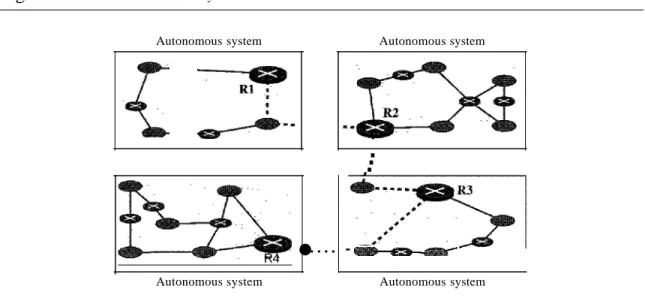
Today, an internet can be so large that one routing protocol cannot handle the task of updating the routing tables of all routers. For this reason, an internet is divided into autonomous systems. Anautonomous system (AS) is a group of networks and routers under the authority of a single administration. Routing inside an autonomous system is referred to as intradomain routing. Routing between autonomous systems is referred to as interdomain routing. Each autonomous system can choose one or more intrado- main routing protocols to handle routing inside the autonomous system. However, only one interdomain routing protocol handles routing between autonomous systems (see Figure 22.12).
Figure 22.12 Autonomous systems
Autonomous system Autonomous system
~A
. . R4.
Autonomous system
···
.... •
_~D-""1IIIIIr'Autonomous system
Several intradomain and interdomain routing protocols are in use. In this section, we cover only the most popular ones. We discuss two intradomain routing protocols:
distance vector and link state. We also introduce one interdomain routing protocol: path vector (see Figure 22.13).
Routing Information Protocol (RIP) is an implementation of the distance vector protocol. Open Shortest Path First (OSPF) is an implementation of the link state proto- col.Border Gateway Protocol (BGP)is an implementation of the path vector protocol.
Figure 22.13 Popular routing protocols
Distance Vector Routing
In distance vector routing, the least-cost route between any two nodes is the route with minimum distance. In this protocol, as the name implies, each node maintains a vector (table) of minimum distances to every node. The table at each node also guides the packets to the desired node by showing the next stop in the route (next-hop routing).
We can think of nodes as the cities in an area and the lines as the roads connecting them. A table can show a tourist the minimum distance between cities.
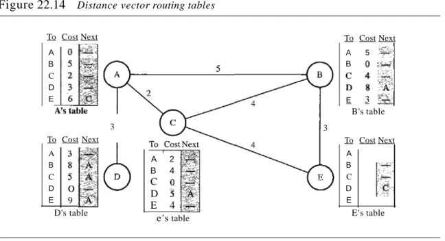
In Figure 22.14, we show a system of five nodes with their corresponding tables.
Figure 22.14 Distance vector routing tables
D's table E's table
To Cost Next A
B C D E
To Cost Next
A 5
¥!:
B () ~W
~
:~~i
E 3 ~~.
B's table 3
e'stable
A 2
B 4
C (}
D '5
E 4
3 <
8 5
o
9
3 A
B C D E A B C D E
To Cost Next To Cost Next
The table for node A shows how we can reach any node from this node. For exam- ple, our least cost to reach node E is 6. The route passes through C.
Initialization
The tables in Figure 22.14 are stable; each node knows how to reach any other node and the cost. At the beginning, however, this is not the case. Each node can know only
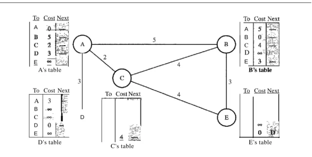
the distance between itself and its immediate neighbors, those directly connected to it.
So for the moment, we assume that each node can send a message to the immediate neighbors and find the distance between itself and these neighbors. Figure 22.15 shows the initial tables for each node. The distance for any entry that is not a neighbor is marked as infinite (unreachable).
Figure 22.15 Initialization of tables in distance vector routing
3 To Cost Next
A -O,'~'i~·
~ n~
E "" f~~~,;:'A's table To Cost Next
A 3
~
B ,'"',
C .>~,~
D
0["
E "" k<7
D's table D
~5:J~
4 (~i C's table
3 A B C
D M
E 3
To Cost Next
QQ ~;" ~~c,'.;
() :jf,
E'stable
Sharing
The whole idea of distance vector routing is the sharing of information between neigh- bors. Although node A does not know about node E, node C does. So if node C shares its routing table with A, node A can also know how to reach node E. On the other hand, node C does not know how to reach node D, but node A does. Ifnode A shares its rout- ing table with node C, node C also knows how to reach node D. In other words, nodes A and C, as immediate neighbors, can improve their routing tables if they help each other.
There is only one problem. How much of the table must be shared with each neighbor? A node is not aware of a neighbor's table. The best solution for each node is to send its entire table to the neighbor and let the neighbor decide what part to use and what part to discard. However, the third column of a table (next stop) is not useful for the neighbor. When the neighbor receives a table, this column needs to be replaced with the sender's name. Ifany of the rows can be used, the next node is the sender of the table. A node therefore can send only the first two columns of its table to any neighbor. In other words, sharing here means sharing only the first two columns.
Indistance vector routing, each node shares its routing table with its immediate neighbors periodically and when there is a change.
Updating
When a node receives a two-column table from a neighbor, it needs to update its rout- ing table. Updating takes three steps:
1. The receiving node needs to add the cost between itself and the sending node to each value in the second column. The logic is clear. Ifnode C claims that its distance to a destination isx mi, and the distance between A and C isymi,then the distance between A and that destination, via C, isx+ymi.
2. The receiving node needs to add the name of the sending node to each row as the third column if the receiving node uses information from any row. The sending node is the next node in the route.
3. The receiving node needs to compare each row of its old table with the correspond- ing row of the modified version of the received table.
a. Ifthe next-node entry is different, the receiving node chooses the row with the smaller cost. If there is a tie, the old one is kept.
b. Ifthe next-node entry is the same, the receiving node chooses the new row. For example, suppose node C has previously advertised a route to node X with dis- tance 3. Suppose that now there is no path between C and X; node C now adver- tises this route with a distance of infinity. Node A must not ignore this value even though its old entry is smaller. The old route does not exist any more. The new route has a distance of infinity.
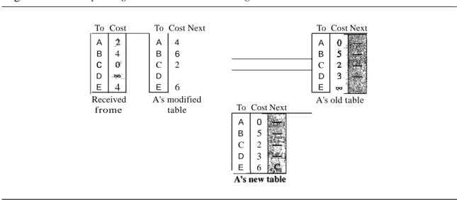
Figure 22.16 shows how node A updates its routing table after receiving the partial table from nodeC.
Figure 22.16 Updating in distance vector routing
To Cost To Cost Next To Cost Next
A ~2 A 4 A 0
B 4 B 6 B .5
c if C 2 C 2
D ,1?0~_ D D '3
E 4 E 6 E qo
Received A's modified A's old table
frome table To Cost Next
A 0
B 5
C 2
D 3
E 6
There are several points we need to emphasize here. First, as we know from math- ematics, when we add any number to infinity, the result is still infinity. Second, the modified table shows how to reach A from A viaC. If A needs to reach itself via C, it needs to go to C and come back, a distance of 4. Third, the only benefit from this updat- ing of node A is the last entry, how to reach E. Previously, node A did not know how to reach E (distance of infinity); now it knows that the cost is 6 viaC.
Each node can update its table by using the tables received from other nodes. In a short time, if there is no change in the network itself, such as a failure in a link, each node reaches a stable condition in which the contents of its table remains the same.
When to Share
The question now is, When does a node send its partial routing table (only two columns) to all its immediate neighbors? The table is sent both periodically and when there is a change in the table.
Periodic Update A node sends its routing table, normally every 30 s, in a periodic update. The period depends on the protocol that is using distance vector routing.
Triggered Update A node sends its two-column routing table to its neighbors any- time there is a change in its routing table. This is called a triggered update. The change can result from the following.
1. A node receives a table from a neighbor, resulting in changes in its own table after updating.
2. A node detects some failure in the neighboring links which results in a distance change to infinity.
Two-Node Loop Instability
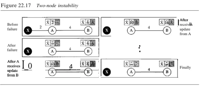
A problem with distance vector routing is instability, which means that a network using this protocol can become unstable. To understand the problem, let us look at the scenario depicted in Figure 22.17.
Figure 22.17 Two-node instability
Before failure
After
failure
·
•·
I
Aft"receivesBupdate from A
g€, I_o ~_-~_~_·· __'__ 4__ ~_'~_'_"_:r-o----~-··~-~-:~-¥,t-: --4--~-X-:-;:-J-I) --,
FinallyFigure 22.17 shows a system with three nodes. We have shown only the portions of the routing table needed for our discussion. At the beginning, both nodes A and B know how to reach node X. But suddenly, the link between A and X fails. Node A changes its table. IfA can send its table to B immediately, everything is fine. However, the system becomes unstable if B sends its routing table to A before receiving A's routing table.
Node A receives the update and, assuming that B has found a way to reach X, immedi- ately updates its routing table. Based on the triggered update strategy, A sends its new
update to B. Now B thinks that something has been changed around A and updates its routing table. The cost of reaching X increases gradually until it reaches infinity. At this moment, both A and B know that X cannot be reached. However, during this time the system is not stable. Node A thinks that the route to X is via B; node B thinks that the route to X is via A. If A receives a packet destined for X, it goes to B and then comes back to A. Similarly, if B receives a packet destined for X, it goes to A and comes back to B. Packets bounce between A and B, creating a two-node loop problem. A few solu- tions have been proposed for instability of this kind.
Defining Infinity The first obvious solution is to redefine infinity to a smaller num- ber, such as 100. For our previous scenario, the system will be stable in less than 20 updates. As a matter of fact, most implementations of the distance vector protocol define the distance between each node to be I and define 16 as infinity. However, this means that the distance vector routing cannot be used in large systems. The size of the network, in each direction, can not exceed 15 hops.
Split Horizon Another solution is called split horizon. In this strategy, instead of flooding the table through each interface, each node sends only part of its table through each interface. If, according to its table, node B thinks that the optimum route to reach X is via A, itdoes not need to advertise this piece of information to A; the information has corne from A (A already knows). Taking information from node A, modifying it, and sending it back to node A creates the confusion. In our scenario, node B eliminates the last line of its routing table before it sends it to A. In this case, node A keeps the value of infinity as the distance to X. Later when node A sends its routing table to B, node B also corrects its routing table. The system becomes stable after the first update:
both node A and B know that X is not reachable.
Split Horizon and Poison Reverse Using the split horizon strategy has one draw- back. Normally, the distance vector protocol uses a timer, and if there is no news about a route, the node deletes the route from its table. When node B in the previous scenario eliminates the route to X from its advertisement to A, node A cannot guess that this is due to the split horizon strategy (the source of information was A) or because B has not received any news about X recently. The split horizon strategy can be combined with the poison reverse strategy. Node B can still advertise the value for X, but if the source of information is A, it can replace the distance with infinity as a warning: "Do not use this value; what I know about this route comes from you."
Three-Node Instability
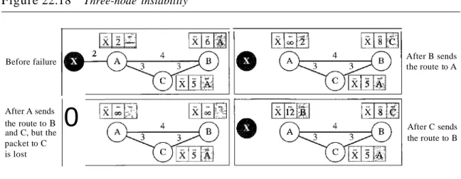
The two-node instability can be avoided by using the split horizon strategy combined with poison reverse. However, if the instability is between three nodes, stability cannot be guaranteed. Figure 22.18 shows the scenario.
Suppose, after finding that X is not reachable, node A sends a packet to Band C to inform them of the situation. Node B immediately updates its table, but the packet to C is lost in the network and never reaches C. Node C remains in the dark and still thinks that there is a route to X via A with a distance of 5. After a while, node C sends to Bits routing table, which includes the route to X. Node B is totally fooled here. Itreceives information on the route to X from C, and according to the algorithm, it updates its
Figure 22.18 Three-node instability
Before failure
After A sends the route toB
0
and C,but the packet to C is lost
[ill8
2 After B sends
the route to A
After C sends the route to B
table, showing the route to X via C with a cost of 8. This information has come from C, not from A, so after awhile node B may advertise this route to A. Now A is fooled and updates its table to show that A can reach X via B with a cost of 12. Of course, the loop continues; now A advertises the route to X to C, with increased cost, but not to B. Node C then advertises the route to B with an increased cost. Node B does the same to A.
And so on. The loop stops when the cost in each node reaches infinity.
RIP
The Routing Information Protocol (RIP) is an intradomain routing protocol used inside an autonomous system. It is a very simple protocol based on distance vector routing. RIP implements distance vector routing directly with some considerations:
1. In an autonomous system, we are dealing with routers and networks (links). The routers have routing tables; networks do not.
2. The destination in a routing table is a network, which means the first column defines a network address.
3. The metric used by RIP is very simple; the distance is defined as the number of links (networks) to reach the destination. For this reason, the metric in RIP is called a hop count.
4. Infinity is defined as 16, which means that any route in an autonomous system using RIP cannot have more than 15 hops.
5. The next-node column defines the address of the router to which the packet is to be sent to reach its destination.
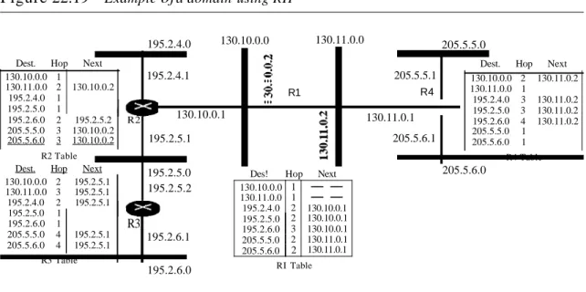
Figure 22.19 shows an autonomous system with seven networks and four routers. The table of each router is also shown. Let us look at the routing table for Rl. The table has seven entries to show how to reach each network in the autonomous system. Router Rl is directly connected to networks 130.10.0.0 and 130.11.0.0, which means that there are no next-hop entries for these two networks. To send a packet to one of the three networks at the far left, router Rl needs to deliver the packet to R2. The next-node entry for these three networks is the interface of router R2 with IP address 130.10.0.1. To send a packet to the two networks at the far right, router Rl needs to send the packet to the interface of router R4 with IP address 130.11.0.1. The other tables can be explained similarly.
Figure 22.19 Example of a domain using RIP
195.2.4.0 130.10.0.0 130.11.0.0 205.5.5.0
Dest. Hop Next 130.10.0.0 2 130.11.0.2 130.11.0.0 1
195.2.4.0 3 130.11.0.2 195.2.5.0 3 130.11.0.2 195.2.6.0 4 130.11.0.2 205.5.5.0 1
205.5.6.0 1 R4 Table 205.5.6.0
205.5.5.1 R4 130.11.0.1
205.5.6.1
RI Table N~
Q
...
~ R1
...
Des! Hop Next 130.10.0.0 1 - -
130.11.0.0 1 - -
195.2.4.0 2 130.10.0.1 195.2.5.0 2 130.10.0.1 195.2.6.0 3 130.10.0.1 205.5.5.0 2 130.11.0.1 205.5.6.0 2 130.11.0.1 130.10.0.1
195.2.5.1 195.2.5.0 195.2.5.2 195.2.4.1
R3
195.2.6.1 195.2.6.0 Dest. Hop Next
R3 Table 130.10.0.0 1
130.11.0.0 2 130.10.0.2 195.2.4.0 1
195.2.5.0 1
195.2.6.0 2 195.2.5.2 R2 205.5.5.0 3 130.10.0.2 205.5.6.0 3 130.10.0.2
R2 Table Dest. Hop Next 130.10.0.0 2 195.2.5.1 130.11.0.0 3 195.2.5.1 195.2.4.0 2 195.2.5.1 195.2.5.0 1
195.2.6.0 1
205.5.5.0 4 195.2.5.1 205.5.6.0 4 195.2.5.1
Link State Routing
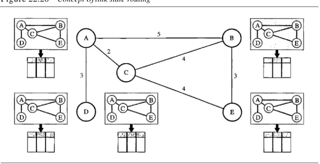
Link state routing has a different philosophy from that of distance vector routing. In link state routing, if each node in the domain has the entire topology of the domain- the list of nodes and links, how they are connected including the type, cost (metric), and condition of the links (up or down)-the node can use Dijkstra's algorithm to build a routing table. Figure 22.20 shows the concept.
Figure 22.20 Concept of link state routing
The figure shows a simple domain with five nodes. Each node uses the same topology to create a routing table, but the routing table for each node is unique because the calcu- lations are based on different interpretations of the topology. This is analogous to a city map. While each person may have the same map, each needs to take a different route to reach her specific destination.
The topology must be dynamic, representing the latest state of each node and each link. Ifthere are changes in any point in the network (a link is down, for example), the topology must be updated for each node.
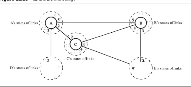
How can a common topology be dynamic and stored in each node? No node can know the topology at the beginning or after a change somewhere in the network. Link state routing is based on the assumption that, although the global knowledge about the topology is not clear, each node has partial knowledge: it knows the state (type, condi- tion, and cost) of its links. Inother words, the whole topology can be compiled from the partial knowledge of each node. Figure 22.21 shows the same domain as in Figure 22.20, indicating the part of the knowledge belonging to each node.
Figure 22.21 Link state knowledge
"
I
A's states of links ~ ,:("'$
-
~.- ..., /'3' '"
I ~
D's states of links~.,
;1
\ I
... ' ~,-,,/
....::; '-,,-C~:,....
C's states ofIinks /'-~3""
I " , , ,
I . \
t4: IE's states ofIinks
,
'.}"
-_.-'
"Node A knows that it is connected to node B with metric 5, to node C with metric 2, and to node D with metric 3. Node C knows that it is connected to node A with metric 2, to node B with metric 4, and to node E with metric 4. Node D knows that it is con- nected only to node A with metric 3. And so on. Although there is an overlap in the knowledge, the overlap guarantees the creation of a common topology-a picture of the whole domain for each node.
Building Routing Tables
In link state routing, four sets of actions are required to ensure that each node has the routing table showing the least-cost node to every other node.
]. Creation of the states of the links by each node, called the link state packet (LSP).
2. Dissemination of LSPs to every other router, called flooding, in an efficient and reliable way.
3. Formation of a shortest path tree for each node.
4. Calculation of a routing table based on the shortest path tree.
Creation of Link State Packet (LSP) A link state packet can carry a large amount of information. For the moment, however, we assume that it carries a minimum amount
of data: the node identity, the list of links, a sequence number, and age. The first two, node identity and the list of links, are needed to make the topology. The third, sequence number, facilitates flooding and distinguishes new LSPs from old ones. The fourth, age, prevents old LSPs from remaining in the domain for a long time. LSPs are generated on two occasions:
1. When there is a change in the topology of the domain. Triggering of LSP dissemi- nation is the main way of quickly informing any node in the domain to update its topology.
2. On a periodic basis. The period in this case is much longer compared to distance vector routing. As a matter of fact, there is no actual need for this type of LSP dis- semination. It is done to ensure that old information is removed from the domain.
The timer set for periodic dissemination is normally in the range of 60 min or 2 h based on the implementation. A longer period ensures that flooding does not create too much traffic on the network.
Flooding of LSPs After a node has prepared an LSP, it must be disseminated to all other nodes, not only to its neighbors. The process is called flooding and based on the following:
1. The creating node sends a copy of the LSP out of each interface.
2. A node that receives an LSP compares it with the copy it may already have.Ifthe newly arrived LSP is older than the one it has (found by checking the sequence number), it discards the LSP.Ifit is newer, the node does the following:
a. Itdiscards the old LSP and keeps the new one.
b. Itsends a copy of it out of each interface except the one from which the packet arrived. This guarantees that flooding stops somewhere in the domain (where a node has only one interface).
Formation of Shortest Path Tree: Dijkstra Algorithm After receiving all LSPs, each node will have a copy of the whole topology. However, the topology is not sufficient to find the shortest path to every other node; a shortest path tree is needed.
A tree is a graph of nodes and links; one node is called the root. All other nodes can be reached from the root through only one single route. A shortest path tree is a tree in which the path between the root and every other node is the shortest. What we need for each node is a shortest path tree with that node as the root.
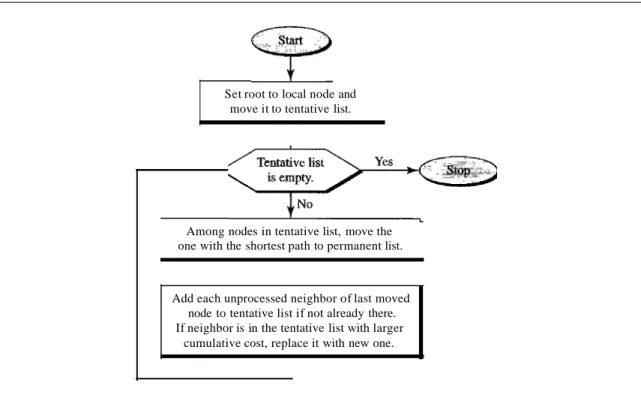
The Dijkstra algorithm creates a shortest path tree from a graph. The algorithm divides the nodes into two sets: tentative and permanent. It finds the neighbors of a current node, makes them tentative, examines them, and if they pass the criteria, makes them permanent. We can informally define the algorithm by using the flowchart in Figure 22.22.
Let us apply the algorithm to node A of our sample graph in Figure 22.23. To find the shortest path in each step, we need the cumulative cost from the root to each node, which is shown next to the node.
The following shows the steps. At the end of each step, we show the permanent (filled circles) and the tentative (open circles) nodes and lists with the cumulative costs.
Figure 22.22 Dijkstra algorithm
Set root to local node and move it to tentative list.
Among nodes in tentative list, move the one with the shortest path to permanent list.
Add each unprocessed neighbor of last moved node to tentative list if not already there.
If neighbor is in the tentative list with larger cumulative cost, replace it with new one.
Figure 22.23 Example offormation of shortest path tree
Root
B 5 0.·~.---{B 5
00
RootI. Set root to A and move A to tentative list.
Root
o .
3
4. Move D to permanent list.
Root
o .
2. Move A to permanent list andadd B, C, and D to tentative list.
5. Move B to permanent list.
Topology
3. Move C to permanent and add E to tentative list.
6 6. Move E to permanent list
(tentative list is empty).
1. We make node A the root of the tree and move it to the tentative list. Our two lists are Permanent list: empty Tentative list: A(O)
2. Node A has the shortest cumulative cost from all nodes in the tentative list. We move A to the pennanent list and add all neighbors of A to the tentative list. Our new listsare
Permanent list: A(O) Tentative list: B(5), C(2),D(3)
3. Node C has the shortest cumulative cost from all nodes in the tentative list. We move C to the permanent list. Node C has three neighbors, but node A is already pro- cessed, which makes the unprocessed neighbors just B and E. However, B is already in the tentative list with a cumulative cost of5. NodeA could also reach node B through C with a cumulative cost of 6. Since 5 is less than 6, we keep node B with a cumulative cost of5in the tentative list and do not replace it. Our new lists are
Permanent list: A(O),e(2) Tentativelist: B(5), 0(3), E(6)
4. Node D has the shortest cumulative cost of all the nodes in the tentative list. We move D to the permanent list. Node D has no unprocessed neighbor to be added to the tentative list. Our new lists are
Permanent list: A(O),C(2), 0(3) Tentative list:B(5), E(6)
5. Node B has the shortest cumulative cost of all the nodes in the tentative list. We move B to the permanent list. We need to add all unprocessed neighbors of B to the tentative list (this is just node E). However, E(6) is already in the list with a smaller cumulative cost. The cumulative cost to node E, as the neighbor of B, is 8. We keep node E(6) in the tentative list. Our new lists are
Permanent list: A(O),B(5), C(2), 0(3) Tentative list: E(6)
6. Node E has the shortest cumulative cost from all nodes in the tentative list. We move E to the permanent list. Node E has no neighbor. Now the tentative list is empty. We stop; our shortest path tree is ready. The final lists are
Permanent list: A(O),B(5), C(2), D(3),E(6) Tentative list: empty
Calculation of Routing Table from Shortest Path Tree Each node uses the short- est path tree protocol to construct its routing table. The routing table shows the cost of reaching each node from the root. Table 22.2 shows the routing table for node A.
Table 22.2 Routing table for node A Node Cost Next Router
A 0 -
B 5 -
C 2 -
D 3 -
E 6 C
Compare Table 22.2 with the one in Figure 22.14. Both distance vector routing and link state routing end up with the same routing table for nodeA.
OSPF
The Open Shortest Path First or OSPF protocol is an intradomain routing protocol based on link state routing. Its domain is also an autonomous system.
Areas To handle routing efficiently and in a timely manner, OSPF divides an auto- nomous system into areas. An area is a collection of networks, hosts, and routers all contained within an autonomous system. An autonomous system can be divided into many different areas. All networks inside an area must be connected.
Routers inside an area flood the area with routing information. At the border of an area, special routers calledarea border routers summarize the information about the area and send it to other areas. Among the areas inside an autonomous system is a spe- cial area called the backbone; all the areas inside an autonomous system must be con- nected to the backbone. In other words, the backbone serves as a primary area and the other areas as secondary areas. This does not mean that the routers within areas cannot be connected to each other, however. The routers inside the backbone are called the backbone routers. Note that a backbone router can also be an area border router.
If, because of some problem, the connectivity between a backbone and an area is broken, a virtual link between routers must be created by an administrator to allow continuity of the functions of the backbone as the primary area.
Each area has an area identification. The area identification of the backbone is zero. Figure 22.24 shows an autonomous system and its areas.
Figure 22.24 Areas in an autonomous system
Area0(backbone)
l-~. To other
ASs
Autonomous system
Metric The OSPF protocol allows the administrator to assign a cost, called themetric, to each route. The metric can be based on a type of service (minimum delay, maximum throughput, and so on). As a matter of fact, a router can have multiple routing tables, each based on a different type of service.
Types of Links In OSPF terminology, a connection is called a link. Four types of links have been defined: point-to-point, transient, stub, and virtual (see Figure 22.25).
Figure 22.25 Types of links
A point-to-point link connects two routers without any other host or router in between. In other words, the purpose of the link (network) is just to connect the two routers. An example of this type of link is two routers connected by a telephone line or a T line. There is no need to assign a network address to this type of link. Graphically, the routers are represented by nodes, and the link is represented by a bidirectional edge connecting the nodes. The metrics, which are usually the same, are shown at the two ends, one for each direction. In other words, each router has only one neighbor at the other side of the link (see Figure 22.26).
Figure 22.26 Point-to-point link
~C"'Il~f-- ~.4~
~ Point-to-point network ~
Router Router
A transient link is a network with several routers attached to it. The data can enter through any of the routers and leave through any router. All LANs and some WANs with two or more routers are of this type. In this case, each router has many neighbors. For example, consider the Ethernet in Figure 22.27a. Router A has routers B, C, D, and E as neighbors. Router B has routers A, C, D, and E as neighbors. Ifwe want to show the neighborhood relationship in this situation, we have the graph shown in Figure 22.27b.
Figure 22.27 Transient link
A
E
c D A
b. Unrealistic representation c. Realistic representation E
B
c D Ethernet
a. Transient network
This is neither efficient nor realistic. Itis not efficient because each router needs to advertise the neighborhood to four other routers, for a total of 20 advertisements. Itis
not realistic because there is no single network (link) between each pair of routers;
there is only one network that serves as a crossroad between all five routers.
To show that each router is connected to every other router through one single net- work, the network itself is represented by a node. However, because a network is not a machine, it cannot function as a router. One of the routers in the network takes this responsibility. Itis assigned a dual purpose; it is a true router and a designated router.
We can use the topology shown in Figure 22.27c to show the connections of a transient network.
Now each router has only one neighbor, the designated router (network). On the other hand, the designated router (the network) has five neighbors. We see that thc number of neighbor announcements is reduced from 20 to 10. Still, the link is repre- sented as a bidirectional edge between the nodes. However, while there is a metric from each node to the designated router, there is no metric from the designated router to any other node. The reason is that the designated router represents the network. We can only assign a cost to a packet that is passing through the network. We cannot charge for this twice. When a packet enters a network, we assign a cost; when a packet leaves the network to go to the router, there is no charge.
A stub link is a network that is connected to only one router. The data packets enter the network through this single router and leave the network through this same router. This is a special case of the transient network. We can show this situation using the router as a node and using the designated router for the network. However, the link is only one-directional, from the router to the network (see Figure 22.28).
Figure 22.28 Stub link
,.
A Ethernet a. Stub networkA
• ""-,,...k' ro_
b. Representation
When the link between two routers is broken, the administration may create a virtual link between them, using a longer path that probably goes through several routers.
Graphical Representation Let us now examine how an AS can be represented graphically. Figure 22.29 shows a small AS with seven networks and six routers. Two of the networks are point-to-point networks. We use symbols such as Nl and N2 for transient and stub networks. There is no need to assign an identity to a point-to- point network. The figure also shows the graphical representation of the AS as seen by OSPF.
We have used square nodes for the routers and ovals for the networks (represented by designated routers). However, OSPF sees both as nodes. Note that we have three stub networks.
Figure 22.29 Example of an AS and its graphical representation in OSPF
1---lII~l----I-1~"- - - - N2
c
Nl a. Autonomous system
B T-31ine
N3--+O--...,£:i"---I N5
b. Graphical representation 8
4
Path Vector Routing
Distance vector and link state routing are both intradomain routing protocols. They can be used inside an autonomous system, but not between autonomous systems. These two protocols are not suitable for interdomain routing mostly because of scalability. Both of these routing protocols become intractable when the domain of operation becomes large. Distance vector routing is subject to instability if there are more than a few hops in the domain of operation. Link state routing needs a huge amount of resources to cal- culate routing tables. It also creates heavy traffic because of flooding. There is a need for a third routing protocol which we callpath vector routing.
Path vector routing proved to be useful for interdomain routing. The principle of path vector routing is similar to that of distance vector routing. In path vector routing, we assume that there is one node (there can be more, but one is enough for our concep- tual discussion) in each autonomous system that acts on behalf of the entire autono- mous system. Let us call it the speaker node. The speaker node in an AS creates a routing table and advertises it to speaker nodes in the neighboring ASs. The idea is the same as for distance vector routing except that only speaker nodes in each AS can com- municate with each other. However, what is advertised is different. A speaker node advertises the path, not the metric of the nodes, in its autonomous system or other autonomous systems.
Initialization
At the beginning, each speaker node can know only the reachability of nodes inside its autonomous system. Figure 22.30 shows the initial tables for each speaker node in a system made of four ASs.
Figure 22.30 Initial routing tables in path vector routing
Dest. Path .A$L2
AS:L.
Al Table AS 1
Des!. Path Bl AS2\
B2