In this thesis we prove that channel models (a)–(d) can be used as input to the generalized Dijkstra algorithm without creating a routing loop. These routing algorithms work by comparing different possible paths from the source to the destination based on their routing statistics.
Generalized Network Routing Metrics
Using these operators, we can then use the Generalized Dijkstra Algorithm (GDA) [8] to find the best path with the smallest p. In the thesis, we prove that these channels are compatible with the generalized Dijkstra algorithm, which means that the algorithm is guaranteed not to create a routing loop.
Generalized Network Routing Algorithms
The only way to keep these tables synchronized is to use message passing algorithms that "flood" the entire network with identical copies of the tables. In this chapter, we also discuss our contribution to the application of the threshold-based message passing algorithm in error correction decoding.
Additional Topics
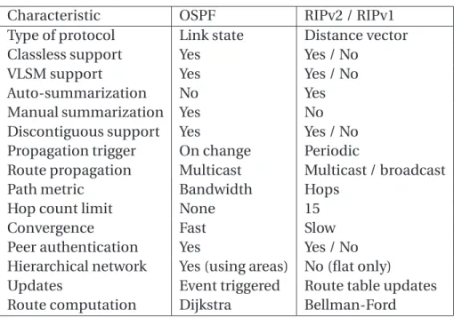
Static routing protocols assume that the routing table—that is, the network "address book" and topology—never changes. Two of the most important classes are the Link State Routing (LSR) and the Distance Vector Routing (DVR) protocols.
Dijkstra’s Algorithm
Relaxation
Using this method, an upper bound[v] on the actual shortest path weight of each node is repeatedly reduced until the upper bound cannot be reduced any further. Before relaxation can be used, the shortest path boundaries and predecessors must be initialized to make π[v]=NIL and l[v]=0 for allv∈V − {s}.
Dijkstra’s Algorithm
At each iteration, the node u∈V−S≡Q that has the smallest shortest path score[u] is inserted into S(and removed fromQ). In each iteration of the while loop, the node u∈Q with the smallest shortest path score is extracted from Q =V−S and moved to S .
Complexity Analysis of Dijkstra’s Algorithm
If the shortest path w.r.t can be improved by passing through u, the values ofl[v] andπ[v] are updated. If the Fibonacci heap is used instead of the binary heap, a running time of O(VlogV+E) is possible.
Generalized Dijkstra’s Algorithm
The total runtime for this deployment is typically given by O((V+ E) logV), orO(ElogV) if all nodes can be reached from the sources. The time complexity of the GDA is of course identical to the original Dijkstra algorithm, namely O(V2).
Engineering Applications of Generalized Routing Metrics
The most promising method uses joint source and channel coding [13–18], in which the coding algorithms are adapted to the channel parameters of the actual path used for data transmission. These parameters can then be fed into the common source-channel encoder at source.
The random variables corresponding to the input and output symbols of X are denoted by X and X′, respectively. If the input symbol is the delete symbol, then by definition 1−p =1, as shown by the bottom horizontal line.

For example, in Figure 3.8, the black lines show all paths from X =0 to X′′=0 that pass through various possible values of X′. If we assume =0, then the factorP(X′=j |X =0) in summary is visualized in Figure 3.8 by the connections from doti =0 in the first column to all points in the second column.
Gilbert Channels
Introduction
GSP also has an alternative formulation that is relevant to the main topic of this section. One example that is particularly relevant to GSP is the Time Windowed Vehicle Routing Problem (VRPTW.
Formulation
A path f∗ solves the GSP specified by U, Cmax, C(s), and the graph G = (V,E,d) if and only if it solves the SPP specified by. For the converse proof, suppose that g∗ solves the SPP, and that g∗ is different from f∗ that solves the GSP.
Algorithm
Since nodess,t,ui, segmentsfi∗ and weightned(fi∗) are all parts of the specification of an SPP (V′,E′,d′)⊆(V,E,d), then erf∗is a solution of SPP specified by G′. At the end of the first step, setV′ and tentatively E′andd′ are obtained for the virtual graph G′.
Numerical Example
Conclusion
Applications of the Gas Station Problem
Formulation and Notation
For π, the path development operatorπ is defined as a concatenation of the above operators: π=vJ◦eJ◦ ··· ◦e1◦v0. With ⊕ we can now define the path quantities xπ,λπ and ¯xπ in the form of the edge quantities nexi, λi and ¯xi by means of a generalized summation: xπ =Lxi, λπ =Lλi and ¯xπ=Lx¯i.
Algorithm
Therefore, to find the minimum path WCE we first calculate the minimum path WCE for each pair of nodes inV′. In lines 8 and 9, impossible edges inE' are pruned and any isolated nodes inV' are removed.
Conclusion
Nikaein, et al., “MA-FEC: a QoS-based adaptive FEC for multicast communications in wireless networks,” Proceeding of IEEE ICC, 2000, vol. For example, Figure 5.1 shows a change in the network topology and the corresponding change in the node coordinates in the two-dimensional parameter space.
Formulation
If the event is related to connectivity, ie. event is inc(v,t), node ∈V•(t) will resend the messages already in its memory to its neighborsN(v,t). On the other hand, if the event is message-driven, ie. event is inm(v,t), then v will resend N(v,t) and storelm in its memory.
The C OUNTER F LOODING Algorithm
Nodes inV•(t) may leave V(t) and become isolated, but when they reenter the network at t′>t they will be inV•(t′). FIGURE5.7 The arrows indicate allowed transitions of the network nodes in the setsV◦(t),V•(t),V(t), andV\V(t) for HDN.
The Chinese Generals Problem
A Simple Example
The problem involves three generals, labeled A, B, and C, connected in the simple triangular network shown in Figure 5.8 above. In Figure 5.11 above, the generals that satisfy the condition(1)=1 are marked with gray circles.
General Result
To prove the above equation, we use the same technique as we used in the previous section. The expression for Fkl from (5.10) can then be substituted into (5.4) to obtain a graph similar to Figure 5.13.
Threshold-Based Message-Passing Algorithms for Decoding
Codes, Combinatorial Designs, and Graphs
Formulated as a graph code, the LS codes can be decoded with a variant of the iterative decoding algorithms used by (LDPC) graph codes. We now provide an example for the standard iterative erase correction algorithm using the simple (7,4) Hamming code – formulated as an LDPC graph code – whose graph is shown in Figure 5.18.
![Graph codes are among the hottest current research topics in coding theory [33]. Some of them – including many linear ones, and the LDPC codes – perform very close to the Shannon Capacity, an impressive feat considering their conceptual simplicity](https://thumb-ap.123doks.com/thumbv2/123dok/10413351.0/152.918.276.695.406.592/research-including-shannon-capacity-impressive-considering-conceptual-simplicity.webp)
Decoding Example
Finally, after the third iteration, all variable nodes are restored to their original values as shown in Figure 5.26. For example, the erase pattern in Figure 5.27a poses no problem, but the one in Figure 5.27b has a stop set.
Algorithm
Fischer, “The Consensus Problem in Unreliable Distributed Systems (A Brief Review),” Lecture Notes in Computer Science, in Proc. Again in Figure 6.2(c) the hypercube is cut along the width direction and finally in Figure 6.2(d) there is a cut along the depth direction.
Introduction
ThusDq(3, 2)M DS is the number of Latin squares of order q, known only for a few values of q. Hence Dq(3, 2)M DS is the number of Latin squares of orderq, which is known only for a fewqs [2].
Definitions
Using the same dice as defined in Example 4, we can see that b1ogg2 are Latin strips and squares, respectively, while the others are not. When we think of a 3×3×3 cube as a stack of three 3×3 squares, we can "shuffle" the stack in three different ways along its height, width, and depth.
Ternary Latin Hypercubes
We then claim that two orthonormal ternary Latinn-cubes can be generated from any ternary Latinn-cube using left and right cyclic shifts. Now we have to prove that the lemma also holds for all ternary Latinn+1-cubes.
Ternary Latin Hypercubes and MDS Codes
From Definition8, f does not represent an MDS code, because it only maps qvectors of lengthk, outside the qkpossible. The distance is still the same even if we permute the symbols in the four coordinates of R0.
Experimental Results
Decentralized Decision Making in the Game of Tic-Tac-Toe
Introduction
Competent Player
Team Infrastructure
The Tic-Tac-Toe Team
Discussion
Conclusion
A simple BEC network
A brief overview of the OSPF protocol is given in the first section of this chapter. For the sake of completeness, we provide a brief review of GDA in the third section of this chapter.
A corrupted JPEG image
The GDA, operating on generalized routing metrics derived from physical layer parameters, can be used with existing routing technologies to improve common source channel coding. Sobrinho, “Algebra and algorithms for QoS path computation and hop-by-hop routing on the Internet,” IEEE/ACM ToN., vol.
A network of communication channels
Finally, each section concludes with a proof showing that the channel is compatible with the GDA properties. In another interpretation, an erasure symbol itself is a "flag" from the channel that an error occurred during transmission.
A 5-ary erasure channel
The input and output symbols of aq-EC are often represented as two columns of q+1 points each. From top to bottom, the dots in the left and right columns represent the input and output letters 0.
A series combination of two 5-ECs
We will prove that X, the series combination of twoq-ECs denoted by X1andX2, is itself aq-EC by showing that X can be defined by an equation similar to (3.1). In the figure, there are three columns of dots: the leftmost column corresponding to the input symbol of X1, the middle column corresponding to either the output symbol of X1 or the input symbol of X2, and the rightmost column corresponding to the output symbol of X2.
Series q -ECs and the equivalent q-EC
⑥ The operator establishes a total order onΛ, i.e. for each pair of elementsa,b∈ Λ, either a b or a b (or both, in which case a =b). From top to bottom, each dot in the left and right dot columns represents the input and output letters 0.
A 6-ary symmetric channel
Visually, it is common to represent a q-SC with two columns of dots drawn so that each dot in the left column is connected to each dot in the right column (and vice versa), as shown in Figure 3.6.
Series q -SCs and the equivalent q-SC
This channel is itself aq-SC, a claim that can be proved by showing that an equivalent error probability pforX can be calculated from the error probabilities sp1andp2forX1andX2. In contrast, as shown in Figure 3.8, derivation of 1−p involves a much smaller number of combinations and can therefore be considered a much simpler approach that can be applied to a general value of q.
As in the case of forq-ECs, the series combination of X1andX2 forms a channel, which we shall denote by X. As in the case of theq-ECs, the most useful definition of pis cast is in terms of the binary operatoro-plus, which is denoted by ⊕, shown in (3.13) that.
⑥ The operator introduces a total order on Λ that categorizes each pair of elementsa,b ∈Λintoa b ora b (or both, in which case a =b). As with the q-ECs, the spaceΛ of the q-SCs is just [0,q−q1]∈R, with defined as the standard operator≤, which satisfies the total order.
A Gilbert channel
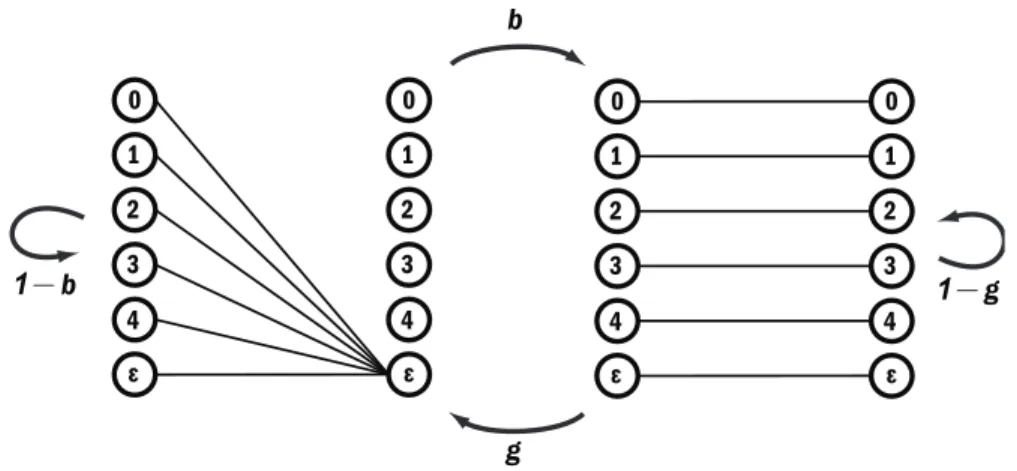
To be consistent, let us denote the random variables corresponding to the input and output symbols of X byX and X′, respectively. Conversely, when the GC is in state G, i.e., when xt =G, the input symbol is identical to the output symbol.
A visual representation of the 5-ary Gilbert channel
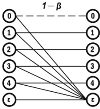
This also means that for a very long string of letters of lengtht, aq-GC, parameterized by (b,g), will look for a β fraction of the time like XB (or the left channel diagram in Figure 3.11). For the remaining fraction of time (which is γ) it will look like XG (or the right channel diagram in Figure 3.11).
A more concise diagram for the 5-ary Gilbert channel
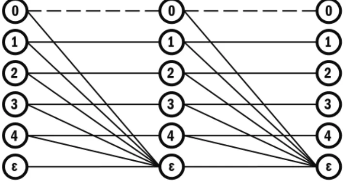
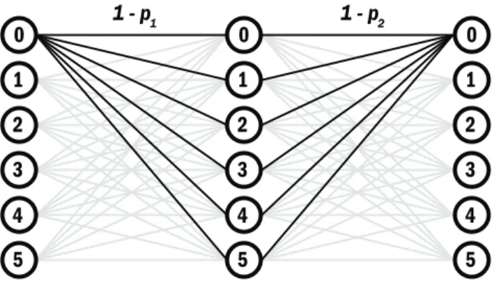
We want to show that the equivalent transition probabilities (b,g) of the series combination, denoted by X, can be calculated from the transition probabilities (b1,g1) and (b2,g2) of the two q-GC components, denoted by X1 and X2. There are three columns of dots in the figure: the leftmost column corresponds to the input symbol X1, the middle column corresponds to the output symbol X1 or the input symbol X2, and the rightmost column corresponds to the output symbol X2. .
A series combination of two 5-GCs
Two independent Gilbert channels
The next equation can be obtained from the definition of the orb, which is best explained by Figure 3.16, which shows two independent Q-GCs operating simultaneously, together with their transitions and probabilities. The second simplest equation turns out to be the definition ofg′ in terms of eg1′ andg2′.
The derivation of g in terms of g 1 and g 2
We can also visually define the shorthand notations for Figures 3.10 and 3.13 in the same way as we defined the ⊕ operator. The abbreviation can make aq-GC look like a typical system element.
Series q -GCs and the equivalent q -GC
In the next subsection, we will discuss the algebraic properties of ⊕and and prove that just like their q-EC counterparts, the twoq-GC operators also satisfy the properties inPand and are therefore compatible with the GDA. Removing two positive terms on the right-hand side does not change the inequality.
Le-Ngoc, “Performance of Future WCDMA Networks Supporting Multimedia Services,” Selected Areas in Communications, IEEE Journal on, vol. 12] Sobrinho, J.L., “Algebra and algorithms for QoS route computation and hop-by-hop routing in the Internet,” IEEE/ACM Transaction on Networking., vol.
A network containing cost-resetting nodes
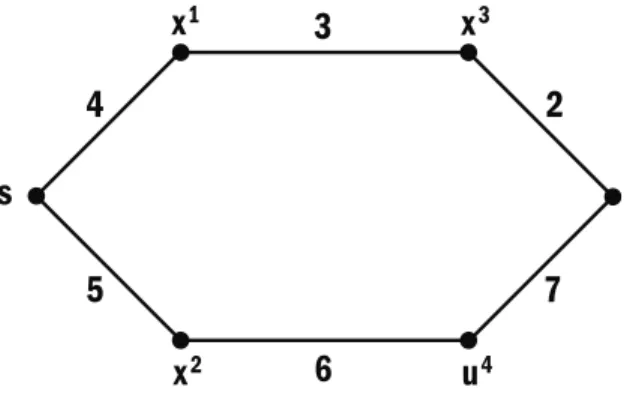
A subset of nodes, ie. The "gas stations", U ⊆V allow a visiting vehicle to refill its on-board fuel to the maximum capacity Cmax. Finally, in the third step on line 11, we obtain the solution f∗(s,t) to the GSP using DA with ∈V′ as the source node.
An example of the Gas Station Problem
Each edge in the network is characterized by the parameter λi of the associated error probability density. In this section, we will analyze the two types of channels that we have discussed extensively in previous chapters: theq-ary symmetric channels (q-SC) and theq-ary sweep channels (q-EC).
The metric space Λ (shaded)
If one (or both) of the vectors is ∞, then by definition of ∞, the sum ⊕ must be ∞. Instead, we find the location of the minimum using the upper and lower bounds of ¡n.
Wang, et al., “A High-Throughput Overlay Multicast Infrastructure with Network Coding,” Proceedings of IFIP IWQOS 2005pp. Since the Internet is a dynamic network with links that change over time, the routers keep their routing tables in sync using message-passing algorithms that "flood" the network with identical copies of the routing table.
Change in network topology and parameter space coordinates
The terms node mobility and edge mobility are defined as the range of capabilities over which nodes and connections can enter and leave the network and change its topology. The theoretical results from this section prove that the explicit set of assumptions used in defining the HDN is also required to guarantee the correctness and termination of the modified flooding algorithm based on the CFA.
The first set contains all nodes that have already been visited by (and thus stored) the message from the source node. The second set contains all nodes that have not yet been visited and are therefore still waiting for the message from the source node.
E(t) is such that each node remains connected to at least one node inV•(t) at all times. The HDN assumption3 generalizes that of the CFAs by introducing a delay between the actual connectivity change∆E(t) and the corresponding eventc(v,t).
Two types of events trigger a message transfer from u to v: (a) when u detects the presence of v at time tc, the event c(u,tc)∈Cui is generated, and (b) when a new message m at time tm arrives and is converted into the setV•(d ,tm), the eventm(u,tm) is generated.
To prove this claim, consider the individual timelines in Figure 5.6, one for each line in E(d,t), all aligned with the markers placed on timet. A message traveling along an edge is represented by an interval [tm,tm+τ] placed on the timeline such that tm ≤t≤tm+τ.
The timelines for E(t ) showing transit and dead regions
Choose two of the timelines with the maximum and minimum values ofm, denoted by tm bytm∗ entm∗, together with the associated intervals. Using the argument above, the dead regions of the maximum and minimum intervals must also overlap because both of them must contain the timestamp+τ.
The arrows indicate allowable transitions of the network nodes in the sets
Using the summary from [20], we can state that BGP assumes the following: (1) there are Sgenerals, of which at most Fgenerals can either maliciously or inadvertently modify a received message before forwarding the message to other generals; (2) all generals have direct access to each other using messengers, ie. the communication network is fully connected; (3) the sender can be identified from the message or message; (4) there is one commanding general who broadcasts the initial message v0 at the beginning of the campaign, and finally, (5) messages are changed only by generals, not by their messengers. Using the next letter in the alphabet (for Albanian and Byzantine), we decide to call our extended problem the Chinese Generals Problem (CGP).
Three generals
Before proceeding to the next subsection for a complete analysis of the CGP, recall that the definition includes the number of generalsS, their valence γ, the initial condition K(0) of the number of generals they decide on A1 and the two tunable parameters M and T indicating the number of sent messengers and the corresponding threshold value, respectively.
Eight possible message configurations
Sixteen possible messenger configurations
Obtaining the new message configurations from the previous messenger
Finally, we can also calculate K(0) and K(1) by counting the numbers of one inv(0) and v(1), which are 2 and 1 respectively. Having defined Fkl, we can now calculate Kk(1), which is the average value of|G1(1)| across all configurations inFk.
The network G with eight generals
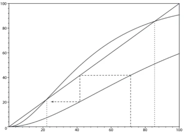
Perhaps unsurprisingly, for Mk ≫1 and γ=S−1, each term in the summation in equation (5.4) is a mathematical expression for the Poisson density Pkl with parameter λ=Mk. These curves can be used to describe the time evolution of Kk(t) and the existence of agreement.
A general γ-regular network
We also note that all γ-regular graphs have the same mgf, and thus the same Fkl, whether they are isomorphic to each other or not.
Two non-isomorphic 4-regular octagonal networks [30, 31]
The q×q entries in aq-ary Latin square lkan are mapped to the symbols of aq-ary codewordc of lengthq2. The entries ofl can also be mapped into the labels of the q2 vertices (the vertices) of a graph g whose adjacent vertices have different labels.
The Tanner graph for the (7,4) Hamming code
Some of them—including many linear and LDPC codes—operate very close to Shannon's performance, an impressive feat given their conceptual simplicity. Second, check nodes in LDPC codes require that variable nodes contain an even (or odd) number of ones.
The (a) q-ary and (b) binary 4 × 4 Sudoku square
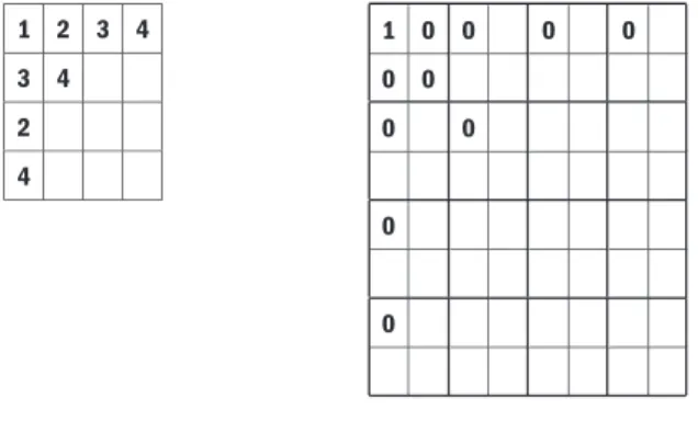
Figure 5.20a is derived from Figure 5.19a and shows only S11 and the other entries of S associated with the Sudoku constraints. Because S11inSi is related to S′11inS′, instead of the q-ary values, Figure 5.20b shows S′111 and the other related binary values Si j k′.
Cellk=1 is on the upper left corner of the subarray and cellk =q is on the lower right corner. Each of the other S′i j ks also has its own limitations hh, hv, hb, andhc (possibly different from S′111s).
Each variable node S′i j k is scrambled in the same structure that enforces codeword integrity, i.e., deleting a symbol affects several control nodes. On the right is the square array Hb with its subsets ordered from upper left to lower right.
One example of a Sudoku puzzle
The variable and check nodes
The puzzle after the first iteration
The puzzle after the second iteration
The puzzle after the third and final iteration
The iterative algorithm we just described inherits the same limitations as the one used to decode erased LDPC ciphers: some puzzles contain stop sets that stop the algorithm prematurely. Once stopped, the algorithm can continue by selecting from (q-ary)S the block, row, or column with the fewest number of deletions and trying all of you.
Squares without and with stopping set
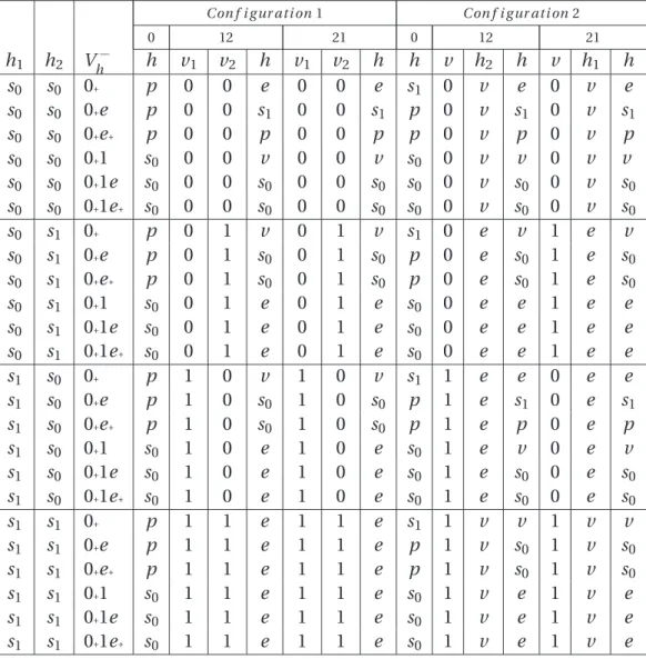
Let V1 and V2 denote two sets of variable nodes, whose binary contents are represented by the vectors V~1 and V~2, respectively. Let H1 and H2 denote two sets of control nodes whose four possible states are stored in the vectors H~1 and H~2, respectively.
The three canonical configurations
Dubois-Ferriere, et al., “Age Matters: Efficient Route Discovery in Mobile Ad-Hoc Networks Using Encounter Age,” Proc. Samar, et al., “Area Independent Routing: An Adaptive Hybrid Routing Framework for Ad Hoc Wireless Networks,” IEEE/ACM TON, vol.
Hypercubes of different dimensions
Without going into too much detail, this aspect of hypercubes can be seen very easily in Figure 6.2. In Figure 6.2(b) we show three slices of this hypercube obtained by cutting the hypercube along its height.
Three different ways to slice a hypercube
Counting the number of q-ary MDS codes of length n and distance d, denoted by Dq(n,d)M DS, is a very difficult problem. This section shows that ford =2, this amounts to counting the number of (n−1)-dimensional Latin hypercubes of ordeq.
Different strips and squares
It simply shuffles the dimension n−1 elements if the shift is on the next coordinate, or applies the shift recursively if . Let's show the effects of cyclic shift operations on the cubes from Example 4.
Three different cyclic shift operations
Next, suppose it is true for ternary Latin dice, that is, ⊲ian =⊲an or⊳an; and⊳ian=⊲anor⊳an. Assume that the formula also holds for ternary Latin cubes, i.e. there are a total of 6· 2n−1 of distinct ain∈ Ln, with i =1.
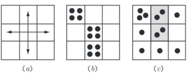
Grid cell numbering convention
Intermediate defensive player
An intermediate attacking player can threaten the opponent with a one-completion attack, thus forcing the opponent to react and defend the position, potentially disrupting any planned movement. An intermediate attacking player will threaten the opponent by placing his piece in cell 1 (or 2), forcing the opponent to occupy cell 2 (or 1).
Intermediate offensive player
A novice offensive player can complete a row when two of its own pieces are already placed in a row with an empty position remaining.
Experienced offensive player
First, let's describe the role of the manager as shown in the algorithm below. Each agent responds with a priority number - saying "let me handle this". In step 4, the manager selects the agent with the highest priority.
Information access rule
In Figure 6.9, the agent is marked with an X, and the cells for which it has complete information are marked with ball symbols.
Novice defensive strategy
Novice defensive play
Failure of the novice defensive strategy
Intermediate defensive strategy
Intermediate defensive play
Novice offensive strategy
Novice offensive play
Intermediate and experienced offensive strategies
Intermediate and experienced offensive play
The T function can be further extended to implement intermediate and experienced attacking strategies, as shown in Figure 13 below. In the next subsection, we discuss several theoretical issues and the question of extending this framework to other types of board games.
Full implementation of the strategy
Initiating a two-completion attack