Networks Second Edition

In field nomenclature, a point is referred to as a node or vertex1 and a line is referred to as an edge. There are a number of practical reasons why we would like to study the network structure of the Internet.

Figure 1.1: The network structure of the Internet. The nodes in this representation of the Internet are “class C subnets”—groups of computers with similar Internet addresses that are usually under the management of a single organization—and the connections

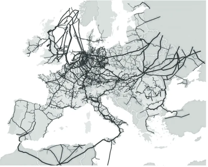
T he I nternet

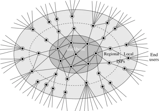
There is currently no simple tool to directly investigate the network structure of the Internet. The third common network granularity is coarse granularity at the level of autonomous systems.

Figure 2.1: A schematic depiction of the structure of the Internet. The nodes and edges of the Internet fall into a number of different classes: the backbone of high-bandwidth long-distance connections; the ISPs, who connect to the backbone and who are div

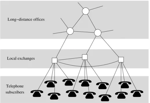
T he telephone network

Individual subscriber telephones are connected to local exchanges, which in turn are connected to remote offices. The remote offices are interconnected by main lines and there may also be some connections between local exchanges.

Figure 2.4: A sketch of the three-tiered structure of a traditional telephone network.

P ower grids

Very comprehensive data on power grids (as well as other energy-related networks such as oil and gas pipelines) is available from specialist publishers, in paper or electronic form, if one is willing to pay for it. Electricity networks also exhibit some unusual behaviors, such as cascading failures, which can lead to surprising results, such as the observed power-law distribution in the size of power outages [140, 263].

T ransportation networks

Just like the Internet, power grids have a spatial element; the individual nodes each have a location somewhere on the globe, and their distribution in space is interesting from geographical, social and economic points of view. Although there is a temptation to apply network models of the kind described in this book to try to explain the behavior of power networks, it is wise to exercise caution.

D elivery and distribution networks

The tree-like structure of the network is clearly visible - there are no loops in the network, so water at each point in the network flows from the plateau through a single path. Also worth mentioning in this area is work on the scaling relationships between the structure of branched vascular networks in organisms and metabolic processes, an impressive example of how an understanding of network structure can be compared to an understanding of function. of systems representing networks.

Figure 2.5: The network of natural gas pipelines in Europe. Thickness of lines indicates the sizes of the pipes.

T he W orld W ide W eb

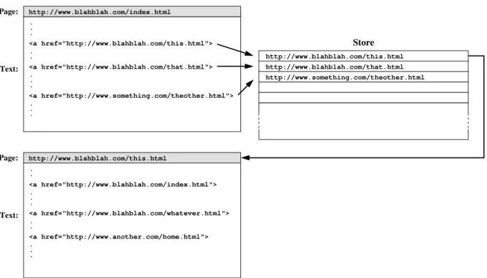
However, perhaps the most important reason why web crawling does not reach every page on the web is that the network structure of the web does not allow it. We do not necessarily rely on search engine companies or other online companies for information about the structure of the web.

Figure 3.1: A network of pages on a corporate website. The nodes in this network represent pages on a website and the directed edges between them represent hyperlinks.

C itation networks

The network's nodes contain information in the form of text and images, just like academic studies of The discussion of citation networks in the previous section focuses on citations between academic articles, but there are other types of citation as well.

O ther information networks

Eliminating central servers and the high-bandwidth connections they require also makes peer-to-peer networks economically attractive in applications such as software distribution. On most peer-to-peer networks, each computer is home to some information, but no one computer has all the information on the network.

T he empirical study of social networks

In this chapter, we provide a discussion of the origins and focus of the field of social network research and describe some of the types of networks we study and the techniques used to determine their structure. The techniques described above, direct questioning of subjects and the use of archival records, are two of the most important, but there are several others that are used regularly.

Figure 4.1: Friendships between schoolchildren. This early hand-drawn image of a social network, taken from the work of psychiatrist Jacob Moreno, depicts friendship patterns between the boys (triangles) and girls (circles) in a class of schoolchildren in

I nterviews and questionnaires

In particular, it clearly limits the out-degree of the nodes in the network, imposing an artificial and possibly unrealistic cutoff. For example, in a study of the social network of a group of doctors, Coleman et al.[117].

D irect observation

One arena where direct observation is essentially the only viable experimental technique is the study of animal social networks, since animals clearly cannot be studied using interviews or questionnaires.

D ata from archival or third - party records

Most of the network data sources considered in this book are not time-resolved, yet many networks change over time. The structure of link networks can be extracted using crawlers similar to those used to search the web—see Section 3.1.

Figure 4.3: Intermarriage network of the ruling families of Florence in the fifteen century

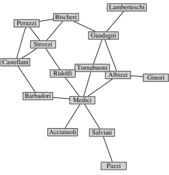
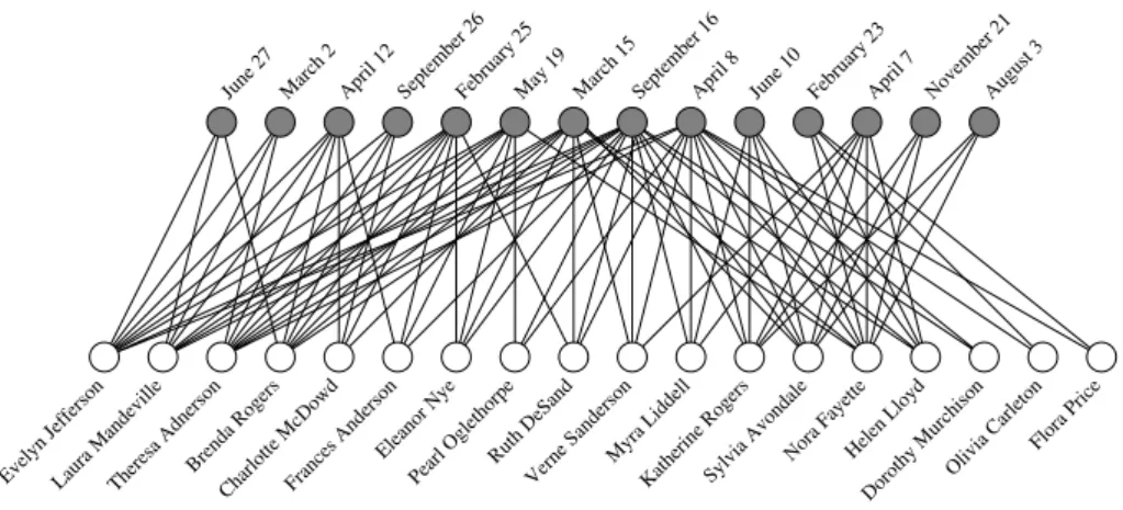
A ffiliation networks

A well-known case is the study by Galaskiewicz [197] of the CEOs of companies in Chicago in the 1970s and their social interaction via clubs they attended: the CEOs are the actors and the clubs are the groups. Also in the business domain, a number of studies have been done of the networks formed by the boards of companies where the actors are company directors and the groups are the boards on which they sit.

T he small - world experiment

Milgram asked the participants to record in the passport each step of the path so he knew how long each path was, and he found that the average length of completed paths from Omaha to the goal in. This result is the origin of the idea of ​​the "six degrees" The phrase "six degrees of separation" did not appear in Milgram's writing.

S nowball sampling , contact tracing , and random walks

You find one initial member of the population of interest and interview them about themselves. Furthermore, random sampling is still not a good technique for testing the structure of the contact network itself.

B iochemical networks

Co-immunoprecipitation is an extension of the immunoprecipitation method for the identification of protein interactions. The amino acid sequence of a protein is determined by a corresponding sequence stored in the DNA of the cell in which the protein is synthesized.

Figure 5.1: Bipartite and tripartite representations of a portion of a metabolic network.

N etworks in the brain

Understanding the structure of neural networks is thus crucial if we want to explain higher-level brain functions. Another type of brain networks are networks of macroscopic functional connectivity between large brain regions.

Figure 5.7: Brain circuitry of a worm. A portion of the neural circuitry of the worm C

E cological networks

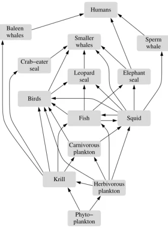
Our food web of Antarctic species is in fact both a shared food web and a food web, as all the species in the network ultimately derive their energy from phytoplankton. An interesting special case of the use of published records is in the construction of paleontological food webs.

Figure 5.9: A food web of species in Antarctica. Nodes in a food web represent species or sometimes, as with some of the nodes in this diagram, groups of related species, such as fish or birds

N etworks and their representation

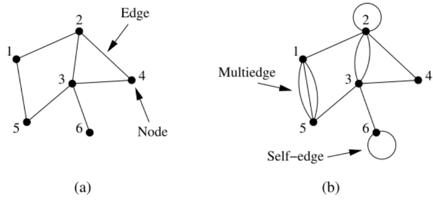
An introduction to the mathematical tools used in the study of networks, tools that will be important for many subsequent developments. Most of the networks we will study have at most a single edge between any pair of nodes.

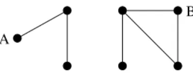
T he adjacency matrix

A network that has neither its own edges nor multiple edges is called simple. It seems not. Two points to keep in mind about the adjacency matrix are, firstly, that for a network like this with no self-edges, all elements of the diagonal matrix are equal to zero, and, secondly, that the matrix is ​​symmetric, since if there is an edge between iandj, then there is necessarily an edge between the jandis.

Figure 6.1: Two small networks. (a) A simple graph, i.e., one having no multiedges or self-edges

W eighted networks

Such edges are represented by setting the corresponding diagonal element of the adjacency matrix equal to twice the multiplicity of the edge: Aii 4 for a double edge itself, 6 for a triple edge, and so on. Thus, one can convert lengths to weights by taking reciprocals and then use those values ​​as elements of the adjacency matrix, although this should only be considered an approximate translation; in most cases there is no formal mathematical relationship between weights and edge lengths.

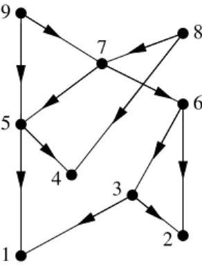
D irected networks

Then somewhere in the network there must be at least one node that has only inbound and no outbound edges. So if the network contains a cycle, there must come a point in our process where there are nodes left in the network, but they all have outgoing edges.

Figure 6.3: A directed acyclic network. In this network the nodes are laid out in such a way that all edges point downward

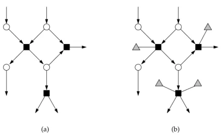
H ypergraphs

These two networks convey the same information - the membership of five nodes in four different groups. a). Bipartite representation in which we introduce four new nodes (open circles at top) representing the four groups, with edges connecting each of the five original nodes (bottom) to the groups to which they belong.

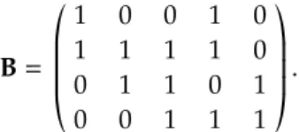
B ipartite networks

At the top and bottom, we show one-mode projections of the network on the two sets of nodes. Mathematically, a one-mode projection can be written in terms of the incidence matrix B of the original bipartite network as follows.

Figure 6.5: A small bipartite network.

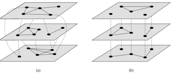
M ultilayer and dynamic networks

There have been many studies of transport networks of the type mentioned above, which are true multi-layer networks, and a number of other examples can be found in the literature. If all parts of the network are trees, the entire network is called a forest.

Figure 6.7: Multilayer and multiplex networks. (a) A multilayer network consists of a set of layers, each containing its own network, plus interlayer edges connecting nodes in different layers (dashed lines)

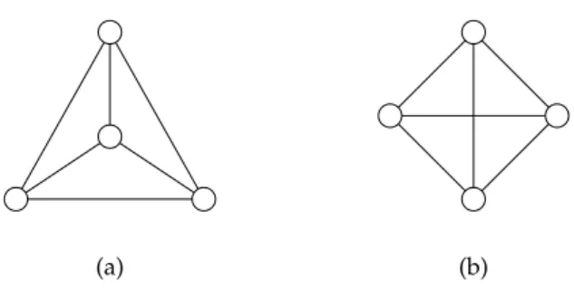
P lanar networks

Another approach would perhaps be to look at the number of occurrences of K5 or UG in the network. In this qualitative sense, "sparse" simply means that most of the possible edges that could exist in the network are not present.

Figure 6.9: Two drawings of a planar network. (a) A small planar network with four nodes and six edges

W alks and paths

Note that this expression counts separately loops consisting of the same nodes in the same order but with different starting points. The expression also counts separately loops consisting of the same nodes, but traversed in opposite directions, so that 1→2→3→1 and 1→3→2→1 are distinct.18 6.11.1 Shortest paths.

C omponents

Technically, a strongly connected component is a maximal subset of nodes such that there is a directed path in both directions between every pair in the subset. Thus, it follows that the out components of all members of a strongly connected component are identical.

Figure 6.13: A network with two com- com-ponents. There is no path between nodes like A and B that lie in different components.

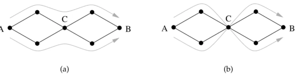
I ndependent paths , connectivity , and cut sets

Cut sets were the focus of an important early result in graph theory. Menger's theorem says that the size of the minimum cut set between any pair of nodes in a network is equal to the number of independent paths between the same nodes. Since the number of independent paths and the size of the cut set are equal, the result follows.

Figure 6.17: Edge independent paths. (a) There are two edge-independent paths from A to B in this figure, as denoted by the arrows, but there is only one node-independent path, because all paths must pass through the center node C.

T he graph L aplacian

Since there are no negative eigenvalues, this is the lowest of the eigenvalues ​​of the Laplacian. The second smallest eigenvalue of the Laplacian is called the algebraic connectivity of the network or the spectral gap.

Figure 6.19: Two visualizations of the same network. In (a) nodes are placed randomly on the page, while in (b) nodes are placed using a network layout algorithm that tries to put connected nodes close to one another, meaning that most edges are short.

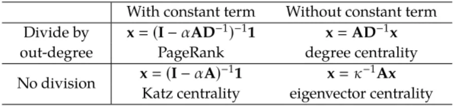
C entrality

This also fixes the value of the constant κ - it must be equal to the largest eigenvalue. In other words, the limiting vector is simply proportional to the leading eigenvector of the matrix.

Table 7.1: Four centrality measures. The four matrix-based centrality measures dis- dis-cussed in the text are distinguished by whether they include an additive constant term in their definition and whether they are normalized by dividing by node degrees

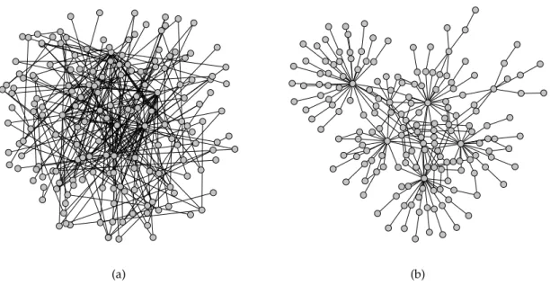
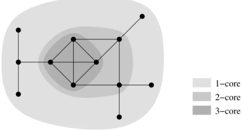
G roups of nodes

An aclique is a set of nodes within an undirected network such that each member of the set is connected by an edge to every other. A component in an undirected network is the (largest) set of nodes such that each is reachable by some path from each of the others.

Figure 7.4: The k-cores in a small network. The shaded regions denote the k-cores for k 1, 2, and 3 in this small network

T ransitivity and the clustering coefficient

An alternative way to write the pooling coefficient is C (number of triangles) × 6. number of paths of length two). Ci (number of neighbor pairs that are connected). the number of pairs of neighbors ofi). 7.29).