I would like to acknowledge the support of the National Science Foundation through a Graduate Research Fellowship. It has been established that there is no significant difference in the average helium amount of the observed associations. For stars with an initial mass in the range of 25 to 60 M0, the evolution of the star is sensitive to the exact rate of mass loss at different evolutionary stages.
Observational Consequences
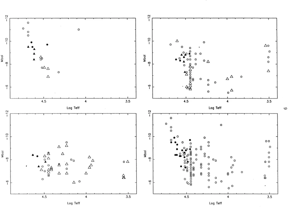
Less massive stars always become red super giants, but if the mass loss rates are low, the star makes a blue loop during the red super giant phase and can cross the Cepheid instability band several times. As in more massive stars, CNO-cycled material appears during the red supergiant phase and causes marked abundance changes. However, for stars of 15 M0 or less, the C/N ratio does not fall below 1 during the first red supergiant phase, and equilibrium amounts of CNO during the loop toward the blue are not yet established.
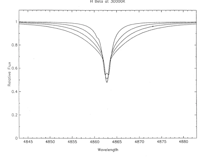
The determination of TeJ J and log g for a sufficiently large sample of stars also allows accurate calibration of the plane mapping (TeJ J, log g) to two-dimensional MK spectral types. This is important for studies in which the observed spectral types are used to construct theoretical temperature-luminosity diagrams for OB associations with known distance moduli [24], [25]. The x2 minimization method was used to determine the selection of stellar parameters, giving the best fit of the theoretical profiles to the observed profiles for each star.
OBSERVATIONS
OBJECT SELECTION
DATA COLLECTION AND REDUCTIONS
The flat field, comparison and spectrograms of the objects were first recreated to remove the curvature from the orders (using the FIGARO CDIST routine). A normalized flat field was then obtained by dividing the raw flat field by a copy of the flat field that had been smoothed in the direction parallel to the order; this ensured that the flatfield was close to unity everywhere (while preserving pixel-to-pixel variations and interference fringes), so that the noisiest, low-signal lines in each order were not artificially amplified when the flatfield was used to calibrate the spectra object. After the observed spectrograms were divided by the normalized flat field, the rows comprising each order were summed and an estimate of the correlation between the orders was subtracted from each order (using the FIGARO routine ECHTRACT).
DATA QUALITY AND SYSTEMATIC ERRORS
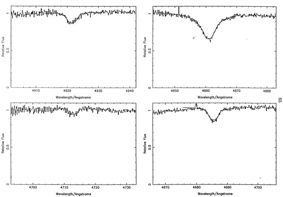
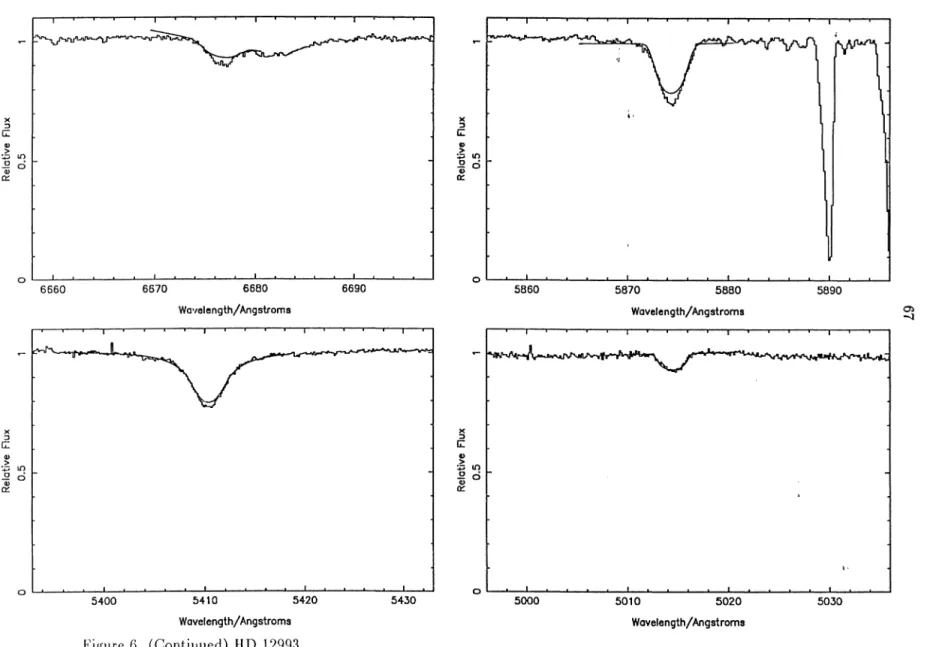
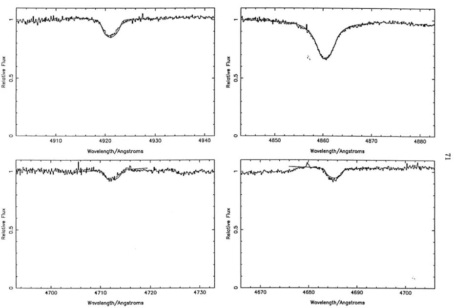
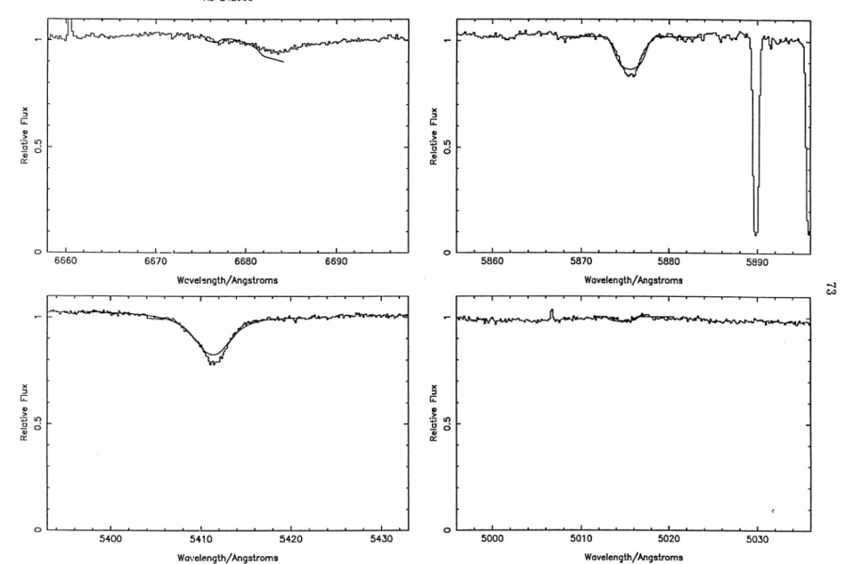
The hydrogen and helium line profiles were obtained by fitting a polynomial to the two orders adjacent to each order containing a line of interest; then the central order was divided by the mean of the two polynomials. In the case of HeI 6678A, a diffuse feature (probably internal to the star rather than an interstellar feature) badly confounds the red arm of the line. Finally, a particular difficulty with echelle spectrograms is the problem of removing the correlation between orders and calculating the scattered light in the instrument.
OBSERVED EQUIVALENT WIDTHS
The equivalent width can then be obtained either by simple integration or by fitting Gaussian profiles. The values quoted here were obtained by simple integration and compared with results from fitting Gaussian profiles to estimate the uncertainties in the values. This allows for the effects of imperfect continuum normalization and mixing and the uncertainty in the Stark-broadened arms of the ionized helium lines.
BACKGROUND
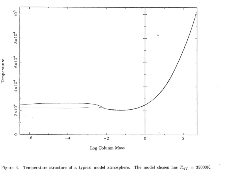
The transfer equation can then be used to determine the perturbations in the radiation field resulting from a perturbation to T; one obtains the equations of the form. The computational cost is dominated by the calculation of the coefficients for equation 5, so that the computational time scales as N D3. The level populations are then revised using the modified mean intensities and temperatures, the transfer equations for all frequencies are solved using the resulting source function, and the distribution of the radiation field in each frequency block is updated.
MODEL ATMOSPHERE AND SYNTHETIC SPECTRUM CALCULATIONS
- Approximations
- The Gray Atmosphere Calculation
- The Non-LTE Calculations
- Computational Costs
- Theoretical Equivalent Widths and Profiles
The gray atmosphere program, GRAY, is a highly modified version of the MAH code written for the same purpose. The effects of the overlapping hydrogen lines are taken into account for the ionized helium lines. All other lines for this model were consistent with those of the adjacent models in the grid.
DETERMINATION OF STELLAR PARAMETERS
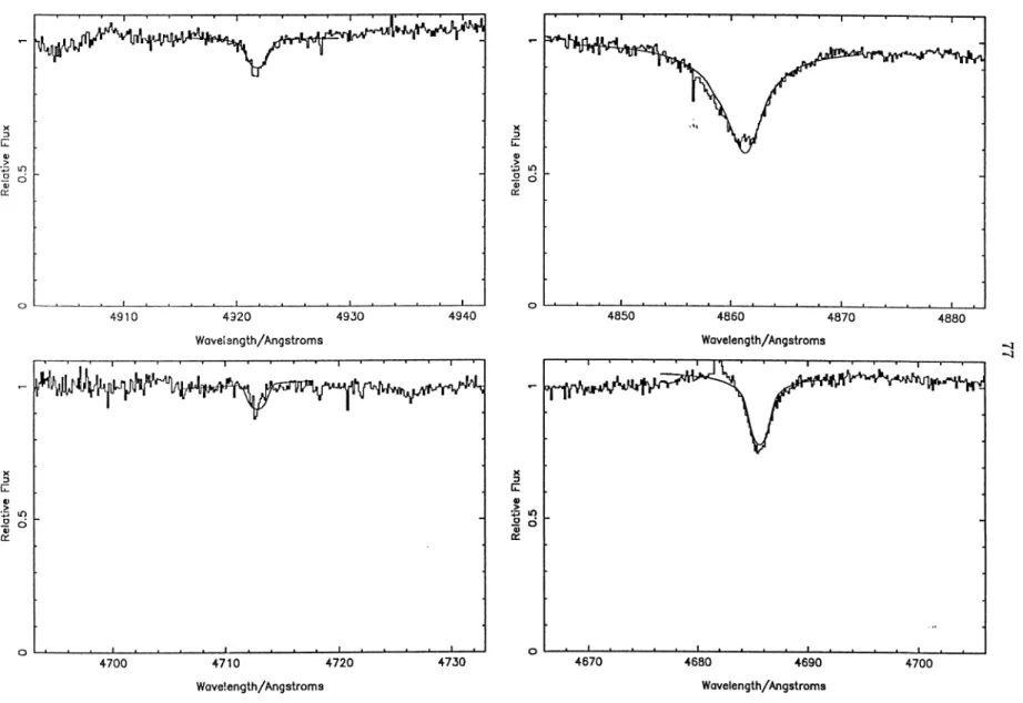
It is clear from these profiles and similarities that the introduction of the three continuum variables was necessary. In most cases, the resulting fits are quite good, especially for the ionized helium lines, indicating that the Schoning-Butler ionized helium profiles are satisfactory. The values of the projected rotational velocity v sin i include the effects of the instrumental profile; given the lowest measured values of v sin i, it seems that rotational speeds of less than about 50 km/s are not resolved.
It is important to determine the ambiguity of the fit (i.e., the range of parameters over which the fit remains good). SPECTRUM quotes errors calculated by determining the change in the parameters that will increase the value of x2 by 30%. These errors appear to be far too conservative; this is understandable, since most of the data points will be insensitive to one or more of the physical.
Another approach is to hold one parameter fixed at a value slightly different from the best fit and recalculate the minimum value with all other parameters allowed to vary. This method was used to determine the errors reported here, where v sin i is a parameter that has been fixed at a non-optimal value. The resulting change in x2 is used to estimate a change in sin i that would significantly degrade the fit, and the corresponding change in the best fit for the physical parameters is reported as error.
In general, the errors thus obtained are close to the scatter one sees in the values of the physical parameters when the fit is repeated for different choices of the portion of the line spectra to fit. Sometimes the errors seem not to be conservative enough; in these cases the error is taken from the scatter in repeated fits, using different portions of the line profiles. It should be emphasized that the cited uncertainties are from the ambiguity of the pass alone;.
CONCLUSIONS
- COMPARISON OF THEORY TO OBSERVATION
- Semi-Empirical Helium Abundances
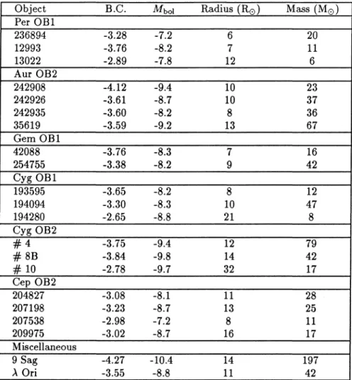
- RADII AND MASSES
- THE MAPPING OF SPECTRAL TYPES TO PHYSICAL PARAMETERS
- SUMMARY
These fitted abundances most likely reflect a systematic failure of the theory rather than the actual composition of the stars involved. However, such a flaw in the theory is not suggested by the quality of the fits, which are generally quite good. The only significant difference between their models and the models used here is the inclusion of the effects of wind blankets.
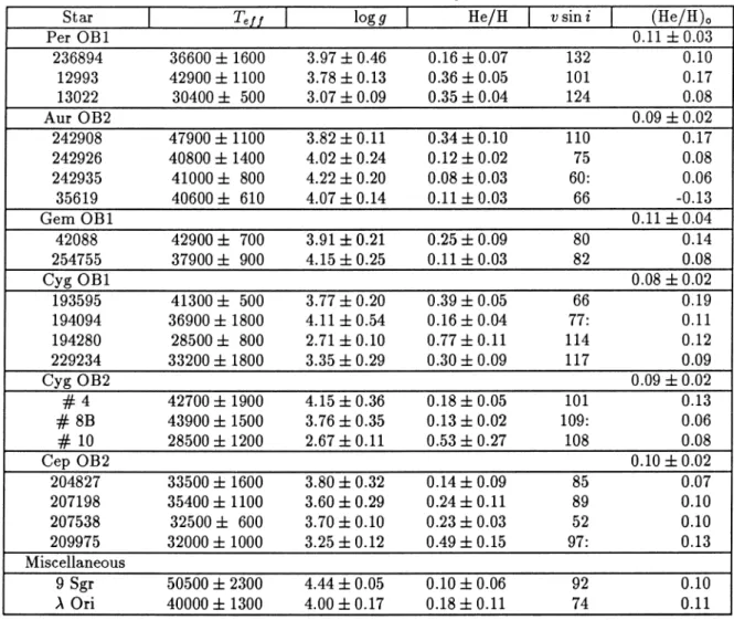
The sensitivity of the hydrogen and helium lines to log g is not large at high Te/I. Unfortunately, due to the paucity of data, our calibration is probably not much more reliable than Humphreys. This mat member was chosen because it is less confused with interstellar scattered bands than the component in 5801A.).
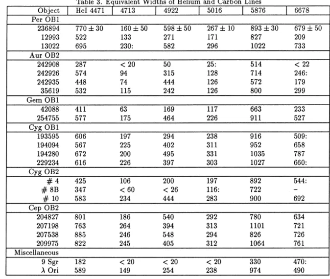
It would be interesting to investigate the nitrogen abundances of the stars in OB2 Cyg as well. Three of the objects for which they present nitrogen spectra are included in the analysis here. A strong correlation exists between the equivalent widths of the CIV 5812A line and the Hell 4342A line.
The following pages list the parts of the FORTRAN source code used to perform the calculations described in this dissertation.
Program GRAY
MAXIMUM HYDROGEI LEVELS FOR PARTITIOI FUICTIOI MAXIMUM HELIUM LEVELS FOR PARTITIOI FUICTIOI BELIUM-2 USES MQB•2 FOR PARTITIOI FUICTIOI IUMBER OF BYDROGELI LEVELS OF TREATELEUMLEUMT TREATED EXPLUS SPIRITUALLY IUMBER OF HELIUM LEVELS OF UNIZED SIIGLY TREATED FAST EXPLOSION COISTAIT OF PLAIK ON THE COISTAI OF BOLTZMAll . BYDROGEI IOIIZATIOI FREQUEICIES IEUTRAL HELIUM IOIIZATIOI FREQUEICIES IOIIZED HELIUM IOIIZATIOI FREQUEICIES BYDROGEI LEVEL STATISTICAL WEIGHTS IEUTRAL HELIUM HELIUM EVENTIEL WEIGHT SURFACE GRAVITY. MASS NETWORK (DIFFERENCES) MEAi MOLECULAR WEIGHT IUCLEI PER PROTOI BYDROGEI IUMBER DEISITY ELECTROI IUMBER DEISITY IEUTRAL HELIUM IUMBER DEISITY IOIIZED HELIUM IUMBERIO DEISITY-IUMBER DEISITY YDROGEI IUMBER DEISITY TOTAL DISTRIBUTION IUMBER DEISITY.
BYDROGEI PBOTOIOIIZATIOI Transverse IEUTRAL HELIUM PBOTOIOIIZATIOI Transverse IOIIZED HELIUM PBOTOIOIIZATIOI Transverse PARTITIOI FUICTIOI BYDROGEI. REAL EXIT, FIT, LEAK, PUTOUT, SETUP, STATE EXTERIAL EXIT, FIT, LEAK, PUTOUT, SETUP, STATE. output, CREATE, TEXT), UIIT6=TERMINAL//"). REAL GFREE, HMFREE EXTERIAL GFREE, HMFREE SRT=1.0/SQRT(TEIIP(ID)) HKT=BK/TEIIP(ID) DO 10 IJ=1,IJ C. HYDROGEI COITRIBUTIOI C.
EXPOIETIALE C TERN REFLECTS C COITRIBUTIOIS WITHOUT UPPER STATE BOUID (BOTH HERE, FOR HELIUM). C GENERAL TABLE OF ACTIVE ELECTROIT QUITUATION OF EACH NEUTRAL STATE C HELIUM TREATED BY THE PROGRAM. C RULE OF SIIIIPSOl; 11 IS THE IUIIBER OF THE CEITRAL FREQUENCY C **IOTE THAT 10 CHECK IS !!ADE TO ENSURE THAT THE TWO FREQUENCY C SUBINTERVALS ARE EQUAL AS THEY SHOULD BE C.**.
C THESE ALLOW INCLUSIONS BOUID LEVELS ABOVE THOSE C EXPRESSLY CONSIDERED AS PART OF FREE-FREE SPACE.
Program LTE
FRE GAUNT
Program ANDERS
ANDERS is listed in its entirety, except for the routines that are essentially identical to those in GRAY and LTE and for a very large number of DATA statements in COLRAT, the inclusion of which would not contribute to the understanding of the program. Al ADAPTATION OF THE PORTIOIS OF THE MIHALAS (1975) CODES TO THE AIDERSOI ALGORITHM FOR EFFICIENT SOLVING OF LARGE IUMBERS OF TRAISFER F.QUATIOIS II 1O1-LTE. MAXIMUM IUMBERS OF FRF.QUEICY BLOCKS MAXIMUM IUMBERS OF DEEP DEPOSITS MAXIMUM TOTAL IUMBERS OF FRF.QUEICIES.
MAXIMUM NUMBER OF HYDROGEN TRAISITIOIS MAXIMUM NUMBER OF JEUTRAL HELIUM TRAISITIOIS MAXIMUM NUMBER OF GEÏOIZED HELIUM TRAISITIOIS MAXIMUM NUMBER OF HYDROGEN NUMBER II PARTITION MAXIMUM NUMBER OF HYDROGEN NUMBER II PARTITION SUM OF HELIUM I TOTAL NUMBER OF ATOMS. POIITS NAAR HYDROGEI LIIE FREQUICIES POIITS NAAR IEUTRAL HELIUM LIIE FRF.QUEICIES POIITS NAAR GEIOIZED HELIUM LIIE FRF.QUEICIES TRAISITIOI IIDICES VOOR HYDROGEI;. TRAISITIOI IIDICES VAN IEUTRAL HELIUM TRAISITIOI IIDICES VAN SIIGLY-IOIIZED HELIUM LAGER NIVEAU VAN DOMIIAIT HYDROGEI TRAISITIOI AT THE.
ITRB IUIIBER OF BYDROGEI TRAISITIOIS ITRBE1 "OF IEUTRAL BELIUII TRAISITIOIS ITRBE2" OF IOIIZED BELIUII TRAISITIOIS. LBS OF POPULATIOI EQUATIOIS RESULT OF POPULATIOI CALCULATIOI B IIATRII OF LIIEARIZATIOI RBS OF POPULATIOI EQUATIOIS C-IIATRII OF LIIEARIZATIOI OPACITY MATRIX. IEUTRAL BELIUII DEISITIES LTE IEUTRAL BELIUII DEISITIES GEIOIZED BELIUII DEISITIES LTE GEIOIIZED BELIUII DEISITIES DOUBLE IOIZED BELIUII DEISITIES FICTIONAL MASSIVE PARTICLE DEISITY PROTOI DEISITY.
LTE DESITES TOTAL PARTICLE DESITES RBS AF LIIARIZATIU IIEA IITEISITY OF RADIATIOI DESITES RADIATIBE BUCKETS NEUTRAL VELIUI ".