The central concept of the course is that dynamical systems are modeled by differential equations. Her doctoral dissertation used partial differential equations to explain the branched structure of the lung.
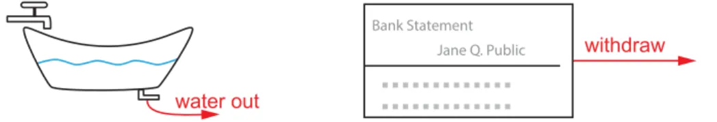
Feedback
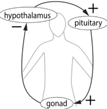
Hormonal regulation Virtually all of the body's hormones are under negative feedback control of the brain and pituitary gland. For example, a protein that is essential in the early development of the embryo is called
Functions
Curly brackets are standard mathematical notation for sets, so here, for example, we're using {drinks} to denote the set of drinks served by the cafe - the domain of this function.). It is important to distinguish between the entire domain of a function and an element of the domain.

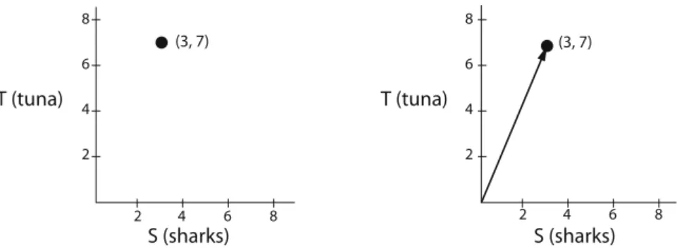
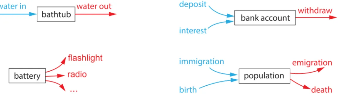
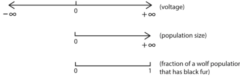
States and State Spaces
For example, the state space for the color of a traffic light is {red, yellow, green}. If the state space is (apples, oranges), we add apples to apples and oranges to oranges.
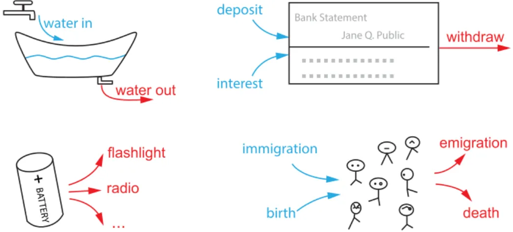
Modeling Change
We will now take up the question of what makes a state point move, that is, the causes of change. The per capita "activation rate," the rate at which latently infected cells become actively infected, is 0.036.
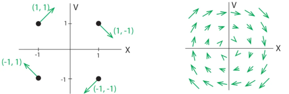
Seeing Change Geometrically
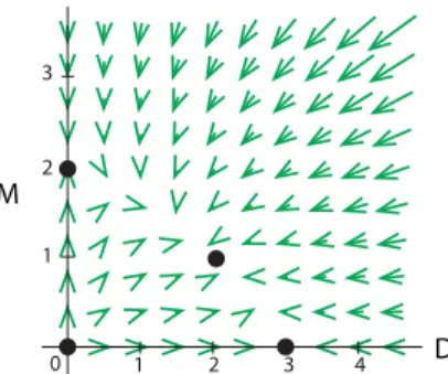
For example, the vector field in Figure 1.39 on the previous page is plotted with the command Sketch the vector field for this system (include your calculations) and describe what happens to each population over time.
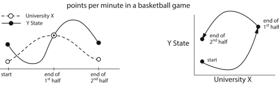
Trajectories
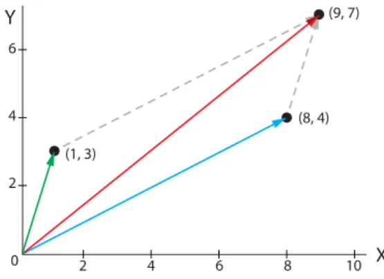
At time 1, which corresponds to the first point in the time series graph, income and expenditure are high. From time series to trajectories and back again We will make heavy use of both time series and state space trajectories. But state-space trajectories carry critical information about the dynamical system, and it is useful to develop the ability to go back and forth between representations of time series and state-space trajectories.
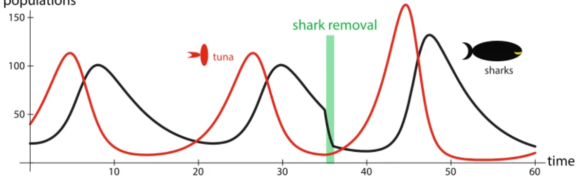
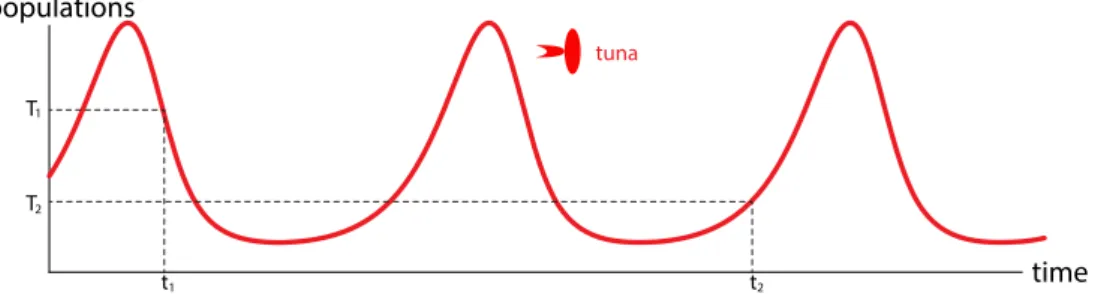
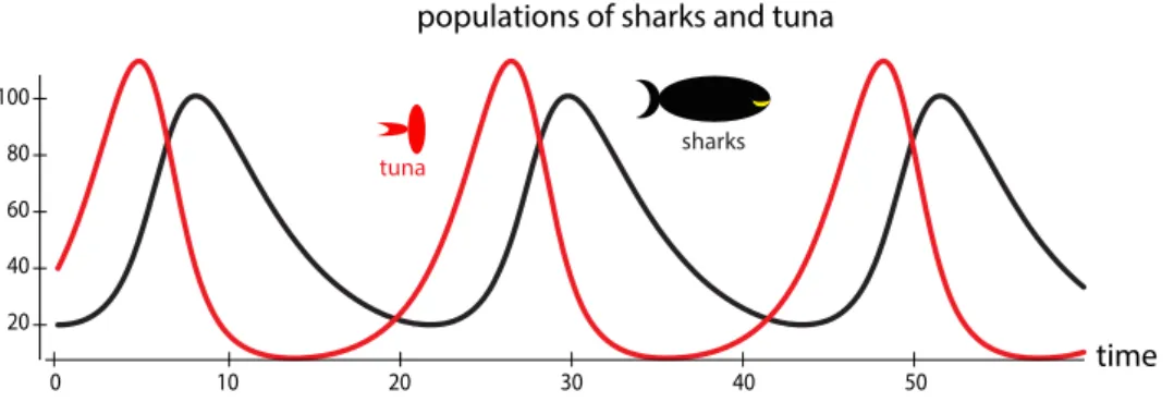
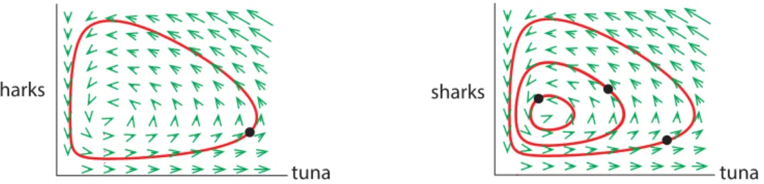
By looking at trajectories in state space, we gain insights into system dynamics that cannot be obtained by looking at individual time series plots. Consider the time series plots for the lynx and snowshoe hare populations in Figure 1.1 on page 1, which we repeat below.
Change and Behavior
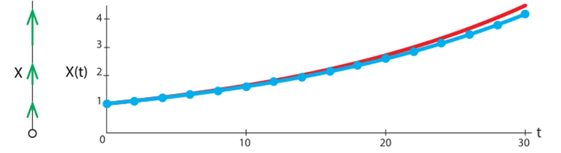
Now we will call newX aboveX1 and one step of Euler's method is complete. The geometric meaning of Euler's method becomes especially clear when we look at the 2D example. The short blue straight lines of Euler's method are too small to see here.
Starting at point X0, one step of Euler's method, with a step size ∆t, (blue arrow), takes the system to point X1. Briefly describe the advantages and disadvantages of using a very small step size in Euler's method.
Derivatives: Rates of Change
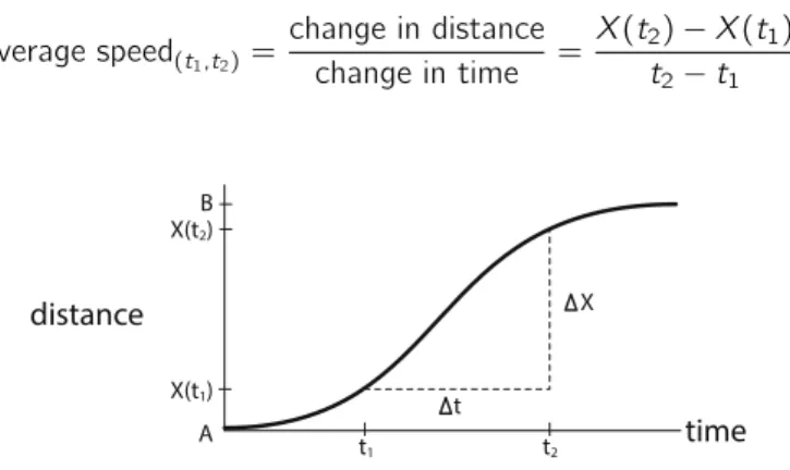
Here the quantity is “distance” and the rate of change of distance with respect to time is called “velocity” or “velocity”. According to the shape of the curve, we can talk about the rate of change of H with respect to M. We can define the concept of the rate of change of P with respect to He exactly as we did when defining the rate of change with respect to time.
We have now defined a concept: for anyY =f(X), at any pointX0, is the instantaneous rate of change of Y with respect to X. We do not yet have a terminology for the instantaneous rate of change with respect to one or other arbitrary variable.
Derivatives: A Geometric Interpretation
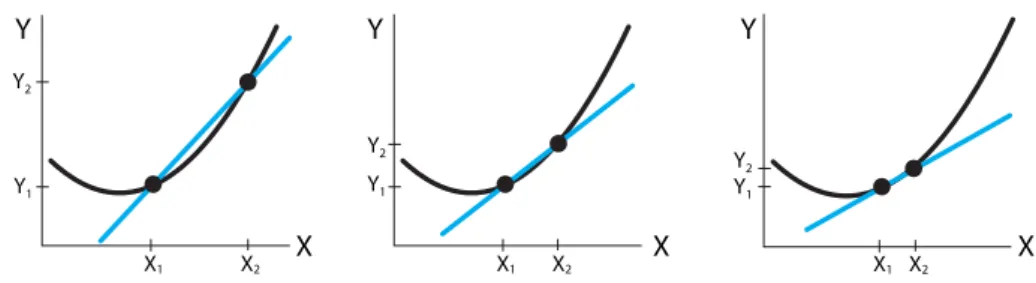
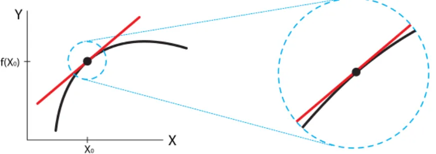
As ∆X gets smaller and smaller, the blue secant lines cut smaller and smaller parts of the curve near X1 (Figure 2.7). As we do this, the blue secant line gets closer and closer to the curve, until finally it approaches a line that "just touches" the curve at the point (X1, Y1).6 This is the line shown in red ( Figure 2.8 ). The tangent is the line whose slope is equal to the derivative of the function at that point.
The most familiar form of the equation for a line is the slope-intercept form (Figure 2.9). This is called the "point-slope" form of the equation for a line, since it explicitly involves the slope and a reference point on the line.
Derivatives: Linear approximation
Since the tangent line is an approximation to a function at a point, we can use it to find approximate values of the function near the point. We cannot even discuss the derivative at the point X= 2 because there is no linear approximation to the right of X = 2 in the function X2, and there is no linear approximation to the left of X = 2 in the function X3. No matter how much we zoom in on X= 2, the function never looks like a straight line through the point.
The lack of a derivative at X = 0 is also clear when we look closely at the function g(X) nearX= 0. Therefore, the function does not have a linear approximation at the corner or at the corner and is not differentiable there (Figure 2. 15).
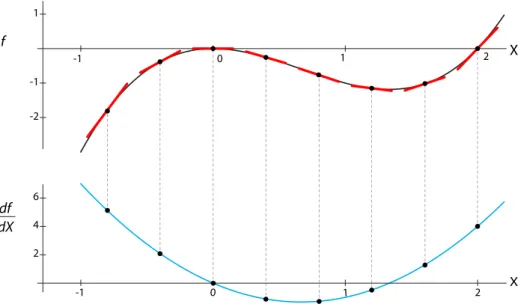
The Derivative of a Function
The answer is yes, and the derivative of the derivative is called this second derivative with respect to X, and is usually written as. Is the second derivative of the function that gives the number of cells positive or negative. For example, to find the derivative of X8, first subtract the 8 in front of the expression, then reduce the exponent to 7, ending up with 8X7.
In other words, the derivative of the sum of two functions is the sum of their derivatives. What is the slope of the tangent to the graph of Y =eX2 atX= 1. Find the linear approximation to the function.
Integration
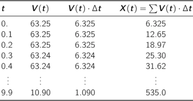
An important class of cases involves a given function f′(t) as a rate of something, and we want to find out the total amount of something deposited by that rate. In other words, the area of the small blue rectangle is the distance traveled during that ∆t. The sum of the small rectangles is approximately the area under the curve, and the sum of the small rectangles is approximately equal to the total distance the car has traveled.
But now let's look at the green rectangle from the point of view of the area-under-f functionF. Referring to the figure, we see that this is the shaded part of the area under the curve D′(t).
Explicit Solutions to Differential Equations
In the year 1256, the Arab scholar ibn Khallikan wrote down the story of the inventor of the game of chess and the Indian king who wanted to reward him for his invention. The inventor asked the king to place one grain of wheat (or, in other versions of the legend, rice) on the first square of the chessboard, two on the second, four on the third, and so on, doubling the number of grains. each subsequent square, until the 64 squares are filled. An exponentially growing population of aardvarks, elephants or naked mole rats would reach the mass of the Earth, then the solar system and finally the universe.
If your roommate takes half the chocolate out of the fridge every night, the fraction of chocolate that remains after a month is smaller than a molecule of chocolate. Mary gives the clerk the dimensions of her pond, and the clerk, knowing the growth rate of the water lilies he has in stock, calculates that if she buys a single water lily, it will produce a population of ten thousand lilies that will replace the entire population of the water lilies will cover. surface of the pond in 20 days.
When X ′ Is Zero
It would be very useful to be able to find that the other behavior was possible, since we cannot run simulations from any initial state.
Equilibrium Points in One Dimension
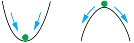
The slope of the tangent tof(X)atX= 0 (the red line passing through X= 0) is positive, soX' goes from negative to positive. We can determine the stability of each of the three by choosing appropriate test points. By drawing representative change vectors on state space, we can easily see the stability of the system's equilibrium points.
Finally, we confirm the linear stability analysis by calculating the sign of the leads at the three equilibrium points. Here we will see why. a) All the following differential equations have an equilibrium point at X = 0.
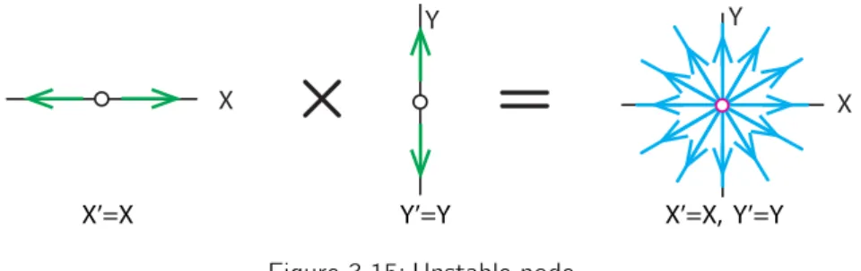
Equilibrium Points in Higher Dimensions
The only way to approach the equilibrium point in the long run is to start right on the stable axis. So far, we have taken two 1D equilibrium points and joined them to make a 2D equilibrium point. Instead, it hangs around the neighborhood of the equilibrium point and oscillates on a new trajectory nearby.
Let's take an unstable spiral inX andY and a stable node inZ, which gives us a 3D unstable equilibrium point. How is each type of equilibrium point you found in the previous part affected by manipulation bandc.
Multiple Equilibria in Two Dimensions
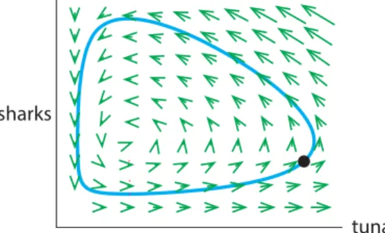
We can use the change vectors on the nullclines to sketch the rest of the vector field. Using the same reasoning, we can sketch the general direction of the change vectors in each of the four regions. Use your sketch of the vector field to determine the type of each equilibrium point.
Use your vector field sketch to determine the type of each equilibrium point. e). Use your vector field sketch to determine the type of each equilibrium point. e).
Basins of Attraction
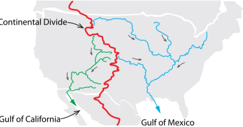
Separating the two is the ridge line of the Rocky Mountains, known as the Continental Divide. Therefore, the Continental Divide divides North America into the two great basins of the Colorado and Mississippi rivers. Each term has the concentration of the protein itself in the numerator, which means that the protein stimulates its own production.
With the usual parameters (see Ingalls (2013)), the zeros of the system look like Figure 3.35, left, and the behavior looks like Figure 3.35, right. The top panel of Figure 3.38 shows the result of applying each of the two signals.
Bifurcations of Equilibria
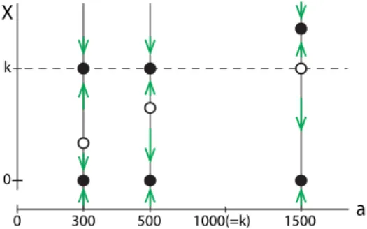
First we will plot different phase portraits at different values of the parameter a, for example 300,500 and 1500. Recall that the points where the red line intersects the black curve are the equilibrium points of the system. For each value of r we place a vertical copy of the state space, where filled points represent the stable equilibrium points and concave points represent the unstable equilibrium points (Figure 3.42).
We can combine this into a picture of the existence and stability of the equilibrium points at different values ofr (Figure 3.44). In this way, the bifurcation diagram gives us a kind of "master view" of the possibilities for intervention in a system.
Oscillations in Nature
Rephrased from “Oscillatory expression of the bHLH factor Hes1 regulated by a negative feedback loop,” by H. Reprinted with permission from AAAS. The clarinetist supplies power to the system by blowing along the long axis of the stick. What actually happens is that if the stick is moving slowly (V is small), then blowing on it will speed it up, so the force of the breath is in the same direction as the movement and adds energy to the system.
There are also better models for musical instruments: we want the character of the musical note to be consistent. This is important because it is the shape of the trajectory that gives the instrument its characteristic sound.
Mechanisms of Oscillation
In the 1970s, it was discovered that the pituitary gland (which is in the head, but not technically in the brain) is actually under the control of the brain. The teenager is trying to keep the car in the center of the lane and the parent tells them to correct right or left, as appropriate. The parent will then start yelling, "go left," the teen will correct again, and the car will rock back and forth, as illustrated in Figure 4.13.
The control of the breathing rate (also called the ventilation rate) is carried out by chemoreceptors in the brain, which send instructions to the nerves that control the lungs. The term "breaths/minute" in the excretion of CO2 from the lungs is the ventilation rateV, which is controlled by the CO2 concentration in the blood.