Electronic Journal of Qualitative Theory of Differential Equations
2008, No. 14, 1-15;http://www.math.u-szeged.hu/ejqtde/
A THIRD-ORDER 3-POINT BVP.
APPLYING KRASNOSEL’SKI˘I’S THEOREM ON THE PLANE
WITHOUT A GREEN’S FUNCTION.
PANOS K. PALAMIDES AND ALEX P. PALAMIDES
Abstract. Consider the three-point boundary value problem for the 3rd
order differential equation:
x′′′(t) =α(t)f(t, x(t), x′ (t), x′′
(t)), 0< t <1, x(0) =x′
(η) =x′′ (1) = 0,
under positivity of the nonlinearity. Existence results for a positive and con-cave solutionx(t), 0 ≤t≤1 are given, for any 1/2 < η <1.In addition, without any monotonicity assumption on the nonlinearity, we prove the exis-tence of a sequence of such solutions with
lim
n→∞||x
n||= 0.
Our principal tool isa very simple applications on a new cone of the plane
of the well-known Krasnosel’ski˘ı’s fixed point theorem. The main feature of this aproach is that, we do not use at all the associated Green’s function, the necessary positivity of which yields the restrictionη∈(1/2,1). Our method still guarantees that the solution we obtain is positive.
1. Introduction
Ma in [21] proved the existence of a positive solution to the three-point nonlinear boundary-value problem
−u′′(t) =q(t)f(u(t)), 0< t <1,
u(0) = 0, αu(η) =u(1),
where α > 0, 0 < η <1 and αη < 1. Later Webb and Infante [14] studied the three-point nonlinear boundary-value problem
−u′′(t) =q(t)f(u(t)), u′(0) = 0, αu′(1) +u(η) = 0
and mainly the loss of positivity of its solutions, asαdecreases. The results of Ma were complemented in the works of Kaufmann [15] and Kaufmann and Raffoul [16]. In the above papers there are no assumptions for singularity of the nonlinearity
f at the pointu= 0. Zhang and Wang [29] and recently Liu [18] obtained some existence results for a singular nonlinear second order 3-point boundary-value prob-lem, for the case where only singularity ofq(t) att= 0 ort= 1 is permitted. Other applications of Krasnosel’ski˘ı’s fixed point theorem to semipositone problems can, for example, be found in [1]. Further recently interesting results have been proved in [4], [11], or [26].
1991Mathematics Subject Classification. Primary 34B10, 34B18; Secondary 34B15, 34G20.
Key words and phrases. three point boundary value problem, third order differential equation, positive solution, vector field, fixed point in cones.
Anderson and Avery [2] and Anderson [3], proved that there exist at least three positive solutions to the BVP (1.1) (below) and the analogous discrete one respec-tively, by using the Leggett-Williams fixed point theorem. Yao in [28] and Haiyan and Liu in [10], using the Krasnosel’ski˘ı’s fixed point theorem showed the existence of multiple solutions to the BVP (1.1). More similar results can be found in Du et al [6] and also in Feng and Webb [7].
Recently, Du et al [5] via the coincidence degree of Mawhin, proved existence for the BVP
(
x′′′(t) =f(t, x(t), x′(t), x′′(t)), 0< t <1,
x(0) =αx(ξ), x′′(0) = 0, x′(1) =Pm−2
j=1 βjx′(ηj),
at the resonance case. In an also recent paper Sun [25], obtained existence of infinitely many positive solutions to the BVP
(1.1)
u′′′(t) =λα(t)f(t, u(t)), 0< t <1, u(0) =u′(η) =u′′(1) = 0, η∈(1/2,1) mainly under superlinearity on the nonlinearityf of the type
There exist two positive constantsθ, R6=rsuch that
f(t, x)≤ r
λM, ∀(t, x)∈[0,1]×[0, r] ;
f(t, x)≥ R
λN, ∀(t, x)∈[0,1]×[θR, R],
whereM andN are also constants. Sun, in order to obtain his existence results ap-plied the classical Krasnosel’skii fixed-point theorem on cone expansion-compression type and furthermore to prove his multiplicity results he assumed monotonicity of the nonlinearity with respect the second variable.
Very recently there have been several papers on third-order boundary value prob-lems. Hopkins and Kosmatov [12], Li [17], Liu et al [19, 20], Guo et al [9] and Kang et al [22] have all considered third-order problems. Graef and Yang [8] and Wong [27] consider three-point focal problems, while Palamides and Smyrlis [23] consider the three-point boundary conditions
u′′′(t) =a(t)f(t, u(t)), x(0) =x′′(η) =x(1) = 0.
In this work, motivated by the above mentioned papers and especially the ones of Sun [25] and Palamides and Smyrlis [23], we suppose a superlinearity-type growth rate of f(t, u, u′, u′′) at both the origin u = 0 and u = +∞. The emphasis in this paper is mainly to apply the well-known Krasnosel’ski˘ı’s fixed point theorem
just on the plane, using in this way an alternative to the classical methodologies, in which as it is common, a Banach space of functions is used. We combine the above Krasnosel’skii’s theorem with properties of the associating vector field, defined on the phase plane and this results in the use of similar quite natural hypothesis.
Furthermore we prove existence of infinitely many positive solutions for the more general boundary value problem
(E)
x′′′(t) =α(t)F(t, x(t), x′(t), x′′(t)), 0< t <1,
x(0) =x′(η) =x′′(1) = 0,
and at the same time, we eliminate at all the related monotonicity assumption on the nonlinearity in [25].
2. Preliminaries
Consider the third-order nonlinear boundary value problem (E), where we as-sume (within this paper) thatη∈(1/2,1),the continuous functionsα(t), t∈(0,1) andF ∈C(Ω,[0,+∞)) are nonnegative and Ω = [0,1]×[0,+∞)×R×(−∞,0].
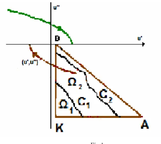
Then, a vector field is defined with crucial properties for our study. More pre-cisely, considering the (x′, x′′) phase semi-plane (x′ > 0), we easily check that
x′′′=α(t)F(t, x, x′, x′′)≥0.Thus, any trajectory (x′(t), x′′(t)), t≥0, emanating from any point in the fourth quadrant:
{(x′, x′′) :x′>0, x′′<0}
“evolutes” in a natural way, when x′(t) > 0, toward the negativex′′−semi-axis. Then, when x′(t)≤0,the trajectory “evolutes” toward the negativex′−semi-axis and finally it stays asymptotically in the second quadrant. As a result, assuming a certain growth rate onf (e.g. a superlinearity), we can control the vector field in a way that assures the existence of a trajectory satisfying the given boundary conditions. These properties, which will be referred as “the nature of the vector field”,combined with the Krasnosel’skii’s principle, are the main tools that we will employ in our study.
Fig 1.
In this paper, we employ a simple cone on the phase plane. First we recall the next definition:
[image:3.595.140.413.425.669.2]Definition 1. Let Ebe a Banach space. A nonempty closed convex set K∗⊂E is
called a cone ofE, iff
(1) x∈K∗, λ >0 ⇒ λx∈K∗;
(2) x∈K∗, −x∈K∗ ⇒x= 0.
For example, the above fourth quadrant ˜
K={(x′, x′′)∈R2:x′≥0, x′′≥0}
on the planeR2 is a cone.
We need a preliminary result from the fixed point theory, which will be our base for all results in this paper.
Precisely will apply the well known Krasnosel’ski˘ı’s fixed point theorem in cones.
Lemma 1. Let E be a Banach space and K∗ ⊂E a cone in E. Assume thatΩ1
andΩ2 are open subsets ofE with0∈Ω1 andΩ1¯ ⊂Ω2.Let
T :K∗∩ Ω2\Ω1¯
→K∗
be a completely continuous operator. We assume furthermore either
(A) ||T u|| ≤ ||u||, ∀u∈K∗∩∂Ω1 and ||T u|| ≥ ||u||, ∀u∈K∗∩∂Ω2 or (B) ||T u|| ≥ ||u||, ∀u∈K∗∩∂Ω2 and ||T u|| ≤ ||u||, ∀u∈K∗∩∂Ω1.
Then T has a fixed point inK∗∩(Ω2\Ω1).
3. Existence Results.
Consider the third-order nonlinear three-point boundary value problem:
(3.1) u′′′ =α(t)f(t, u, u′, u′′), 0< t <1,
(3.2) u(0) =u′(η) =u′′(1) = 0. wheref is a continuous extension of F,i.e.
f(t, u, u′, u′′) =
F(t, u, u′, u′′), u≥0, u′′≤0;
F(t, u, u′,0), u≥0, u′′≥0;
F(t,0, u′,0), u <0, u′′>0;
F(t,0, u′, u′′), u <0, u′′<0.
Remark 1. By the sign property ofF, it follows that
f(t, u, u′, u′′)≥0, (t, u, u′, u′′)∈[0,1]×R3.
Lemma 2. Let u= u(t), t ∈ [0,1] be a solution of the boundary value problem (E) such that
(3.3) u(0) = 0, u′(0) =u′
0>0 and u′′(0) =u′′0 <0.
Then
u(t)≥0, t∈[0,1]
for any initial value(u′
0, u′′0)with u′′0 ≥ −2u′0.
Proof. By the Taylor’s Formula
u(t) =tu′0+
t2 2u ′′ 0+ t3 2 Z 1 0
(1−s)2α(st)F[st, u(ts), u′(ts), u′′(ts)]ds, t∈[0,1].
and (3.3), we getu(t)>0 for alltin a (right) neighborhood oft= 0.Assume that there exists at∗∈(0,1) such that
u(t∗) = 0 and u(t)≥0, t∈[0, t∗]. Given thatu′′
0 ≥ −2u′0,we get, noticing the sign of the nonlinearity
t∗ 2 (2u
′
0+t∗u′′0)≤0 ⇔ t∗ ≥ − 2u′
0
u′′ 0
≥1,
a contradiction.
Assume throughout of this paper, that 0 < θ < 1/2 and there exist positive constantsr0 andR0 with
r0 1 +η2≤ηR0, such that for every 0< r≤r0and anyR≥R0,
(A1)
(
f(t, x, y, z)< r
M, (t, x, y, z)∈∆1, with
∆1= [0,1]×[0, r]×[−r01+η 2
η ,
(1+η2 )r0+R0
η ]×[−
(1+η2 )r0
η ,0];
(A2)
(
f(t, x, y, z)> R
N, (t, x, y, z)∈∆2, with
∆2= [0,1]×[θR,+∞)×[−r01+η 2
η ,
(1+η2 )r0+R0
η ]×[−
(1+η2 )r0
η ,+∞],
where
M =
Z 1
0
α(s)ds >0 and N=
Z 1−θ
θ
α(s)ds >0
Proposition 1. For every initial value (u′
0, u′′0), with u′′0 ≤ −r01+η 2
η <−r0 ≤
−u′
0,any solution u=u(t)of the initial value problem (3.1),(3.3) satisfies
u′(η)<0, and u′′(t)<0, t∈[0,1].
Proof. We choose (without loss of generality)
(3.4) u′
0=r0 and u′′0 =−r0 1 +η2
η
(then u′′
0+ 2u′0 ≤0) and assume that u′′(1) > 0. Since by Remark 1 it follows thatu′′′(t)>0,the function u′′(t), t∈[0,1] is nondecreasing. Hence there exists a t∗∈(0,1) such that
−r0 1 +η2
η ≤u
′′(t)<0, t∈[0, t∗) and u′′(t∗) = 0.
Furthermore,
u′(t)≥ −r01 +η 2
η t≥ −r0
1 +η2
η , t∈[0, t
∗ ).
Thus by the mean value theorem,
0 =u′′(t∗) =u′′ 0+t∗
Z 1
0
α(st∗)f[st∗, u(st∗), u′(st∗), u′′(st∗)]ds.
Now since the derivativeu′(t), t∈[0, t∗) is decreasing, we obtainu′(t)≤u′ 0, t∈ [0, t∗). Hence u(t) < t∗u′
0 ≤ u′0 = r0, t ∈ [0, t∗). Consequently in view of the Remark 1 and the assumption (A1), we obtain the contradiction
u′′(t∗)≤u′′ 0+t∗
r0
M Z 1
0
α(st∗)ds≤u′′
0+t∗r0< u′′0+r0≤0.
On the other hand, again by Taylor’s formula and condition (A1),
u′(η) =u′
0+ηu′′0+η2
R1
0 (1−s)α(sη)f[sη, u(sη), u
′(sη), u′′(sη)]ds
< u′
0+ηu′′0+η2r0= 0.
We recall choices (3.4) andr0 1 +η2≤ηR0 and fix the obtained initial point
K= (u′
0, u′′0).Furthermore consider the simplexS = [K, A, B],where the vertices
A= (u′
A, u′′0) andB= (u′0,0) are chosen so that
(3.5) u′
A+u
′′
0 =η−1R0>0 i.e. u′A=
1 +η2
r0+R0
η .
Proposition 2. The derivative of every solutionu=u(t)of (3.1) emanating from any initial point P1 = (u′1, u′′1)∈ [A, B] (we denote in the sequel such a choice by
u∈ X(P1)) satisfies
u′(t)>0, 0≤t≤η.
Proof. We assume on the contrary thatu′(η)≤0 and notice that
(3.6) u′
1+ηu′′1 >0, for everyP = (u′
1, u′′1)∈[A, B].Indeed, since
u′′ 1=
r0 1 +η2(u′1−r0)
r0η−r0(1 +η2)−R0
, r0≤u′1≤
r0 1 +η2+R0
η ,
it follows that
u′
1+ηu′′1 = u′1
"
1 + ηr0 1 +η 2
r0η−r0(1 +η2)−R0
#
− ηr
2 0 1 +η2
r0η−r0(1 +η2)−R0
= r0
"
1 + ηr0 1 +η 2
r0η−r0(1 +η2)−R0
#
− ηr
2 0 1 +η2
r0η−r0(1 +η2)−R0 =r0>0.
Consider now the two possible cases:
• Let u′′(1) <0. Since obviouslyu′′(t) <0, 0 ≤t ≤ 1, the map u′(t) is decreasing and thus there is a pointt∗∈(0, η] such that
u′(t∗) = 0 and u′(t)≥0, 0≤t≤t∗.
This clearly implies that u(t) ≥0, 0 ≤t ≤t∗ and furthermore we have
f[t, u(t), u′(t), u′′(t)] ≥0. In view of (3.6) and Taylor’s formula, we get the contradiction
u′(t∗) = u′
1+t∗u′′1+t∗2
Z 1
0
(1−s)α(st∗)f[st∗, u(st∗), u′(st∗), u′′(st∗)]ds
> u′
1+ηu′′1>0.
• Let us assume now thatu′′(1)≥0.Then there exists a ˆt∈(0,1] with
u′′ tˆ
= 0 and u′′(t)≤0, 0≤t≤ˆt.
As above we conclude immediately that the function u′(t), 0 ≤t≤ˆt is decreasing. If u′ ˆt
> 0, then, in view of the nature of vector field, we obtainu′(t)>0, 0≤t≤1, a contradiction tou′(η)≤0. Henceu′ tˆ
≤0
and thus we get a pointt∗≤ˆtsuch that
u′(t∗) = 0 andu′(t)≥0, 0≤t≤t∗.
Then as above, Taylor’s formula also leads to another contradictionu′(t∗)> 0.
Lemma 3. Consider a functiony∈C(3)[(0,1),[0,+∞)]such that
y(0) = 0, y′(0)>0 and y′′(0)<0 and
y′′′(t)≥0, 0< t <1, y′(η)≤0 and y′′(1)≤0.
Then
min
θ≤t≤1−θy(t)≥θ||y||, where||y||= max0≤t≤1y(t).
Proof. Sincey′′′(t)≥0, the functiony′′(t) is nondecreasing. So noticingy′′(1)≤0, this implies that
y′′(t)≤0, 0< t <1.
Now due to the concavity ofy(t), for anyµ, t1 andt2 in [0,1],we have
y(µt1+ (1−µ)t2)≥µy(t1) + (1−µ)y(t2).
Moreover using the assumptiony′(η)≤0, we conclude that there is a t∗ ∈(0, η) such thaty′(t∗) = 0 and||y||=y(t∗).Therefore
y(t)≥ ||y|| min
θ≤t≤1−θ
t t∗,
1−t
1−t∗
≥ ||y|| min
θ≤t≤1−θ{t,1−t}=θ||y||.
The next result is crucial for the sequence of our theory.
Lemma 4. Assume that a solutionu=u(t)of a BVP (3.1),(3.2) satisfies moreover the inequalities
u′(t)>0, 0≤t < η and u′′(t)<0, 0≤t <1.
Then
u(t)≥0, 0≤t≤1.
Proof. Suppose that there is aT ∈(η,1) such that
u(t)>0, t∈(0, T), u(T) = 0 andu(t)<0, t∈(T,1].
Sinceη ∈(1/2,1),we get 2η−T ≥0.Consider then, two symmetric with respect toη,partitions
{2η−T =r0< r1< ... < rk =η} and {η=t0< t1< ... < tk=T}
of [2η−T, η] and [η, T] respectively, i.e.
rk−rk−1=t1−t0, rk−1−rk−2=t2−t1, ..., r1−r0=tk−tk−1.
The mapu=u′′(t), t∈[0,1] is nondecreasing and thus we get
u′(r
i)>−u′(tk−i), (i= 0,1, ..., k−1).
So
−(tk−i+1−tk−i)u′(tk−i)<(ri+1−ri)u′(ri), (i= 1,2, ..., k),
reduces to
(3.7) −
k
X
i=1
(tk−i+1−tk−i)u′(tk−i)< k
X
i=1
(ri+1−ri)u′(ri).
In addition, since the mapu′ =u′(t), 0≤r≤T is continuous (and bounded), we can choose the max{ri−ri−1:i= 1,2, ..., k}small enough and given that 2η−T ≥ 0,we obtain
Z η
0
u′(t)dt≥
Z η
2η−T
u′(t)dt >−
Z T
η
u′(r)dr.
Consequently
u(T) =
Z η
0
u′(t)dt+
Z T
η
u′(r)dr >0,
a contradiction.
Remark 2. The restriction η ∈ 1 2,1
is necessary for the validity of the above Lemma 4. Indeed, for η = 1/3 and f(t, u) = 1, the function u(t) = t3/6
−
t2/2
+(5t/18)is a solution of the BVP (3.1)-(3.2), which satisfies the assumptions of Lemma. Butu(1) =−1/18<0.
Proposition 3. Any solution u=u(t) of (3.1) emanating from the above initial point A= (u′
A, u′′0)(with (3.5) to hold) satisfies
||u|| ≥θR0, u′(η)>0 and u′′(1)≥0.
Proof. We will show (extending partially the conclusion of previous Proposition 2) first that
u′(t)> η−1R
0, 0≤t≤1.
If not, then proceeding as in the proof of Proposition 2, we haveu′(t∗) =η−1R 0for somet∗ ∈(0,1], u′(t)≥η−1R
(3.5))
u′(t∗) = u′A+t
∗
u′′0+t ∗2Z
1
0
(1−s)α(st∗)f[st∗, u(st∗), u′(st∗), u′′(st∗)]ds
> u′
A+u′′0 =η−1R0. Hence, given thatu′(t)≤u′
A, 0≤t≤1, we obtain
η−1R
0≤u′(t)≤
1 +η2
r0+R0
η and u(t)>0, 0≤t≤1
and this yields
u(t) =
Z t
0
u′(s)ds≥η−1tR 0.
Moreover, since the mapu=u(t), 0≤t≤1 is nondecreasing, we obtain min
θ≤t≤1−θu(t) =u(θ)≥η
−1θR
0≥θR0.
Consequently, sinceu(t)≥θR0 andu′′(t)≥ u′′0 =−r01+η 2
η , θ≤t≤1−θ,in
view of the assumption (A2),
u′′(1) = u′′ 0+
Z 1
0
α(s)f[s, u(s), u′(s), u′′(s)]ds
> u′′ 0+
Z 1−θ
θ
α(s)f[s, u(s), u′(s), u′′(s)]ds≥u′′
0+R0≥0.
Remark 3. We need some concepts, in the sequel, concerning the case where initial value problems have not a unique solution. Consider a set-valued mappingF,which maps the points of a topological spaceX into compact subsets of another one Y. F
is upper semi-continuous (usc) at x0 ∈ X iff for any open subset V in Y with F(x0) ⊆ V, there exists a neighborhood U of x0 such that F(x) ⊆ V, for every
x∈U. Let P be any initial point such that every solution u∈ X(P) is defined on the interval [0, η]. Then, by the well-known Knesser’s property (see [13, 24]), the
cross-section
X(η;P) ={u(η), u′(η), u′′(η)) :u∈ X(P)}
is a continuum (compact and connected set) in R3, the same being its projections
{u′(η) :u∈ X(P)} and {u′′(1) :u∈ X(P)}. Furthermore the image of a
contin-uum under an upper semi-continuous mapKis again a continuum. Also considering the set-valued mapping
K: Ω→R, K(P) ={u′(η) :u∈ X(P)}
we notice (see[24]) that it is an upper semi-continuous mapping. Obviously, if an IVP has a unique solution, then this map is simply continuous.
Remark 4. By Propositions 1 and 3, there always exist points P1, P2 ∈ [K, A]
such that u′(η) = 0, u ∈ X(P1) and u′′(1) = 0, u ∈ X(P2) respectively. That
conclusion follows immediately by the Remark 3.
In this way, we consider the three-dimensional simplex (triangle)Swith vertices
K = (u′
0, u′′0), A = (u′A, u
′′
0) and B = (u′0,0), under the choices (3.4)-(3.5). The next result is also of central importance for the sequel.
Lemma 5. Let P1= (u′0, u′′1)be a point in the face[K, B]such thatu′(η) = 0,for
some solutionu=u(t)emanating from the initial pointP1i.e. u∈ X(P1). Then
u′′(1)≤0.
Proof. We notice firstly that such a pointP1always exists, because of Propositions 1 and since by the sign of the nonlinearity, u(η)>0 for everyu∈ X(B). Indeed in view of the Remark 3, the image of the segment [K, B] under the mapX, that is
X(η; [K, B]) =∪ {X(η;P) :P ∈[K, B]}
is a continuum. Hence its projection {u′(η) :u∈ X(P) :P ∈[K, B]} crosses the negativeu′−semi axis of the phase-plane.
Next we shall show (following the proof of Proposition 1 and improving partially its conclusion) that, if
u′0=r0 and u′′1 ≤ −r0, (P1= (u′0, u′′1)) then (ifu′′(1) = 0,we have nothing to prove)
u′′(1)<0.
Indeed, by the definition of the modification f, it follows (see Remark 1) that
u′′′(t)>0 and so the functionu′′(t) t∈[0,1] is nondecreasing. Assume now, on the contrary, that u∈ X(P1) is a solution of the differential equation (3.1) such, that u′′(1)>0 (andu′(η) = 0). Hence there exists a t∗∈(0,1) such that
−r0 1 +η2
η ≤u
′′(t)<0, t∈[0, t∗) and u′′(t∗) = 0.
Furthermore
u′(t)≥ −r 0
1 +η2
η t >−r0
1 +η2
η , t∈[0, t
∗).
Also, since the derivativeu′(t), t∈[0, t∗) is decreasing, we obtainu′(t)≤u′ 0, t∈ [0, t∗) and sou(t)< t∗u′
0≤u′0=r0, t∈[0, t∗).Thus by the mean value theorem,
0 =u′′(t∗) =u′′ 1+t∗
Z 1
0
α(st∗)f[st∗, u(st∗), u′(st∗), u′′(st∗)]ds
and in view of the assumption (A1), we obtain the contradiction
u′′(t∗)≤u′′ 1+t∗
r0
M Z 1
0
α(st∗)ds≤u′′
1+t∗r0< u′′1+r0≤0. Assuming now thatu∈ X(P1) implies that u′′(1)>0,we must have (3.8) u′0+u′′1≥0 and (recall) u′0=r0
(since, the inequalityu′′
1 <−u′0, yieldsu′′(1)<0). Also, given thatu′(η) = 0, by the nature of the vector field (sign off), it follows that
u′(t)≥0 and u(t)≥0, 0≤t≤η.
Consequently by the Taylor’s formula, (3.8) and Lemma 2, we get the final contra-diction
u′(η) = u′
0+ηu′′1+η2
Z 1
0
(1−s)α(sη)f[sη, u(sη), u′(sη), u′′(sη)]ds
> u′
0+ηu′′1 ≥u′0+u′′1 ≥0,
due to the properties of the nonlinearity and the assumptionη∈(1/2,1).
Consider now the cone inR2,
K∗=
(u′, u′′)∈R2: u′≥0, u′′≥0 and define the sets (see Fig 1)
Ω1 = {P= (u′
1, u′′1)∈K∗:u′(t)<0, η≤t≤1 andu′′(1)<0, ∀u∈ X(P+K)},
C1 = {P = (u′1, u ′′
1)∈clΩ1:∃ u∈ X(P+K) with u
′(η) = 0 and u′′(1)≤0 }. and also =∂Ω1 C2=∂Ω2
Ω2 = {P = (u′
1, u′′1)∈K∗: u′′(t)<0, 0≤t≤1, ∀u∈ X(P+K)} and
C2 = {P= (u′1, u′′1)∈clΩ2:∃ u∈ X(P+K) with u′(η)≥0 and u′′(1) = 0 },
where we recall once again thatK= (u′ 0, u′′0) =
r0,−r01+η 2
η
.
Recalling the Remark 3, we state the next
Proposition 4. The setΩi is open and ∂Ωi⊆Ci (i= 1,2).
Proof. Assume that the set Ω1is not open and consider anyP0∈Ω1∩∂Ω1.Then, noticing the definition of Ω1, it follows that u′(t) < 0, η ≤ t ≤ 1, for every
u∈ X(P0+K),thus
K(P0) ={u′(η) :u∈ X(P0)} ⊂(−∞,0) =V.
The upper semicontinuity of the mapK yields the existence of an open ballU(P0) centering atP0,such that for allP ∈U(P0)
K(P) ={u′(η) :u∈ X(P)} ⊂(−∞,0) =V. But this clearly means that
(3.9) u′(η)<0, ∀u∈ X(U(P)).
Hence P0 is an interior point of Ω1, that is Ω1 is an open set, a contradiction. Similarly someone can prove that Ω2 is also open.
On the other hand, ifP0∈∂Ω1 andP0∈/C1,then any solutionu∈ X(P0+K) yields u′(η)6= 0. To be definite, letu′(η) <0. Then, as we demonstrated above, (3.9) remains true and henceU(P)⊆Ω1. ConsequentlyP0∈/∂Ω1, a contradiction. We may study the caseu′(η)>0, in the same manner indicated above.
Remark 5. By their definition, it is clear thatΩ1¯ ⊆Ω2.Furthermore, Proposition 1 and the choice of the pointK yields 0∈Ω1. Under the assumptionC1∩C26=∅
and noticing Lemma 5 and Remark 4, we get∅6=C1⊆Ω2 andC26=∅and hence Proposition 4 yieldsΩ2\Ω1¯ 6=∅. We finally remark that the sets C1 and C2 may not be so simple as in Fig 1.
Theorem 1. Under assumptions (A1) and (A2), the boundary value problem (E)
admits at least one positive and concave solution.
Proof. We notice first that, ifC1∩C2 6=∅the BVP (3.1),(3.2) clearly accepts a solution. So assumeC1∩C2=∅.Since Ω1and Ω2are open, by Lemma 5, it follows that ¯Ω1⊆Ω2.Now for any pointP = (u′
1, u′′1), we define the map
T : ˜K∩ Ω2\Ω1¯
→K, T˜ (P) = (−u′(η) +u′
1, u′′(1) +u′′1),
where the solution u = u(t) has its initial value at the point P +K, i.e. u ∈ X(P+K).Also recall that
˜
K=
(u′, u′′)∈R2:u′ ≥0 andu′′≥0
denotes the usual cone inR2. The mapT is well defined, that isT(P)∈K,˜ since
P ∈K˜ ∩ Ω2\Ω1¯
implies that u′′(1)≤0 and henceu′(η)≤u′(0) =u′ 1,i.e.
(3.10) −u′(η) +u′
1≥0. Considering now a pointP ∈∂Ω1⊆C1, we have
||T(P)||=| −u′(η) +u′
1|+|u′′(1) +u′′1| ≥ |u1′|+|u′′1|=||P||, due to the facts thatu′(η) = 0, u′′(1)≤0 andu′′
1 ≤0. Similarly, ifP ∈∂Ω2⊆C2,we obtain
||T(P)||=| −u′(η) +u1|+|u′′(1) +u′′1| ≤ |u ′ 1|+|u
′′
1|=||P||, due to the fact thatu′(η)≥0 and (3.10).
Finally, by an application of the Lemma 1, we obtain a fixed point of T in ˜
K ∩(Ω2\Ω1), that is a solution of the BVP (3.1),(3.2). But this solution, by Lemma 4, is a positive one and noticing the modificationf of the nonlinearity, it follows that it is actually a solution of the original equation (E)
Corollary 1. Suppose that
lim
x→0+0max≤t≤1
f(t, x, y, z)
x = 0 and x→lim+∞0min≤t≤1
f(t, x, y, z)
x = +∞.
for all (y, z) in any compact subset of R2. Then the BVP (3.1),(3.2) has at least one positive solution.
Proof. Via the superlinearity atx= 0 assumption, for M1 >0, there isr0>0 such that for any r ≤r0,it follows that f(t, x, y, z)/x < 1/M, for every (t, x, y, z)∈ ∆1, where ∆1 has been defined at the assumption (A1) and R0 therein will be defined below. Hence
f(t, x, y, z)< x M ≤
r
M, (t, x, y, z)∈∆1.
Similarly by the superlinearity of f at infinity, for 1/θN > 0 there exists R0 >
r0, such that for everyR≥R0, f(t, x, y, z)/x >1/θN, (t, x, y, z)∈∆2,that is
f(t, x, y, z)> x θN ≥
θR θN ≥
R
N, (t, x, y, z)∈∆2.
Consequently assumptions (A1)−(A2) are fulfilled and so Theorem 1 guarantee the result.
4. Multiplicity Results
Theorem 2. Suppose that assumptions (A1) and (A2) hold true. Then there exists
a sequence {un} of bounded and positive solutions to the BVP (E), such that
lim||un||= 0. .
Proof. Since, by the nature of the vector field, for anyu∈ X(B) we haveu′(η)>0 and u′′(1)>0, in view of the continuity of solutions upon their initial values, we can find a sub-triangle
[K∗, A∗, B]⊆[K, A, B] with the face [K∗, A∗] parallel to [K, A] such, that
(4.1) u′(η)>0 and u′′(1)>0, u∈ X(P), P ∈[K∗, A∗, B]. We setK∗= (r
0,uˆ′′0) and consider a new simplex [K1, A1, B1] with
K1 =
r1,−r11 +η 2
η
, B1= (0, r1,0) and
A1 =
1 +η2
r1+R0
η ,−r1
1 +η2
η !
(then [K1, A1] is parallel to [K, A]) under the choice
(4.2) r1∈(0, r0) and −r11 +η 2
η >uˆ
′′ 0.
Then in view of assumptions (A1 ) and (A2 ), we may apply once again the Kras-nosel’ski˘ı’s theorem on the triangle [K1, A1, B1],to obtain another positive solution
u= u2(t) of the BVP (3.1),(3.2). By the construction of [K1, A1, B1] and (4.1), it is obvious that u=u2(t) is different than the solution u=u1(t), 0 ≤t ≤1, obtained in the previous Theorem 1.
If we continue this procedure, choosing the sequence{rn} such that limrn= 0,
we may easily obtain a sequence{un} of solutions to the BVP (E). Furthermore,
by the boundary condition (3.2), we obtain
0 =u′
n(η) =u
′
n(0) +ηu
′′
n(0) +η2
Z 1
0
(1−s)α(sη)f[sη, u(sη), u′(sη), u′′(sη)]ds
and so
0 =u′
n(η)≥u′n(0) +ηu′′n(0)
that is
u′
n(0)≤ −ηu
′′
n(0), n= 1,2, ...
By the above procedure (see (4.2)) and especially since limrn = 0,we obtain
limu′′
n(0) = 0
and given thatu′
n(t)≤u′n(0), 0≤t≤η,we finally get
limun(η) = lim[u′n(0) +
Z η
0
u′
n(t)dt]≤lim (1 +η)u
′
n(0) = 0,
that is lim||un||= 0.
5. Discussion
If we assume that both functions α(t) and f(t, x, y, z) are negative, we may easily demonstrate similar existence and multiplicity results. Indeed, considering the (x′, x′′) face semi-plane (x′ ≤0), we easily check thatx′′′ =α(t)f(t, x, x′, x′′)< 0.Thus, any trajectory (x′(t), x′′(t)), t≥0, emanating from any point in the second quadrant
{(x′, x′′) :x′<0, x′′>0}
“evolutes” in a natural way, when x′(t) < 0, toward the positive x′′−semi-axis and then, when x′(t)≥0 toward the positive x′−semi-axis. As a result, under a certain growth rate onf , we can control the vector field in a way that assures the existence of a trajectory satisfying the given boundary conditions. Let’s notice that in present situation, the obtaining solution (x′(t), x′′(t)) is convex, in contrast to the previous case, where it is concave (see Fig. 1).
Furthermore we could easily get analogous results, for the case when the nonlin-earity is sublinear.
References
[1] R. P. Agarwal, S. R. Grace and D. O’Regan; Semipositone higher-order differential equations,
Appl. Math. Lett.17(2004), 201-207.
[2] D. Anderson and R. Avery; Multiple positive solutions to third-order discrete focal boundary value problem,Acta Math. Appl. Sinica.19(2003), 117-122.
[3] D. Anderson; Multiple Positive Solutions for Three-Point Boundary Value Problem,Math. Comput. Modelling 27(1998)49-57.
[4] Z. Bai, Z. Gu and W. Ge; Multiple positive solutions for some p-Laplacian boundary value problems,J. Math. Anal. Appl.300(2005) 81–94.
[5] Z. Du, G. Cai and W Ge, Existence of solutions a class of third-order nonlinear boundary value problem,Taiwanese J. Math.9No 1(2005) 81-94.
[6] Z. Du, W Ge and X. Lin, A class of third-order multi-point boundary value problem, J. Math. Anal. Appl.294(2004), 104-112.
[7] W. Feng and J. Webb, Solvability of three-point boundary value problem, at resonance,
Nonlinear Anal. Theory, Math Appl.30(1997) 3227-3238.
[8] J. R. Graef and B. Yang, Positive solutions of a nonlinear third order eigenvalue problem,
Dynamic Sys. Appl.,15(2006) 97–110.
[9] L. J. Guo, J. P. Sun, and Y. H. Zhao, Existence of positive solutions for nonlinear third-order three-point boundary value problem,Nonlinear Anal., (2007) doi:10.1016/j.na.2007.03.008. [10] H. Haiyan and Y. Liu, Multiple positive solutions to third-order trhee-point singular
bound-ary value problem,Proc Indian Acad. Sci.114No 4(2004), 409-422.
[11] X. He and W. Ge; Twin positive solutions for the one-dimensional p-Laplacian boundary value problems,Nonlinear Analysis 56(2004) 975 – 984.
[12] B. Hopkins and N. Kosmatov, Third-order boundary value problems with sign-changing so-lutions,Nonlinear Analysis,67:1(2007) 126–137.
[13] L. Jackson and G. Klaasen, A variation of Wa˙zewski’s Topological Method,SIAM J. Appl. Math.20(1971), 124-130.
[14] G. Infante and J. R .L. Webb, Loss of positivity in a nonlinear scalar heat equation,NoDEA Nonlinear Differential Equations Appl.13(2006), no. 2, 249–261.
[15] E. R. Kaufmann; Positive solutions of a three-point boundary value on a time scale,Electron. J. of Differential Equations,2003(2003), No. 82, 1-11.
[16] E. R. Kaufmann and Y. N. Raffoul; Eigenvalue problems for a three-point boundary-value problem on a time scale,Electron. J. Qual. Theory Differ. Equ.2004(2004), No.15, 1 - 10.
[17] S. H. Li, Positive solutions of nonlinear singular third-order two-point boundary value prob-lem,J. Math. Anal. Appl.,323(2006) 413–425.
[18] B. Liu; Positive Solutions of Three-Point Boundary-Value Problem for the One Dimensional p-Laplacian with Infinitely many Singularities,Applied. Mathematics Letters17(2004),
655-661.
[19] Z. Q. Liu, J. S. Ume, and S. M. Kang, Positive solutions of a singular nonlinear third-order two-point boundary value problem,J. Math. Anal. Appl.,326(2007) 589–601.
[20] Z. Q. Liu, J. S. Ume, D. R. Anderson, and S. M. Kang, Twin monotone positive solutions to a singular nonlinear third-order differential equation, J. Math. Anal. Appl., 334(2007)
299–313.
[21] R. Ma; Positive solutions of a nonlinear three-point boundary-value problem,Electron. J. of Diff. Eqns,1999(1999), No.34, 1-8.
[22] P. Minghe and S. K. Chang, Existence and uniqueness of solutions for third-order nonlinear boundary value problems,J. Math. Anal. Appl.,327(2007) 23–35.
[23] A. P. Palamides and G. Smyrlis, Positive solutions to a singular third-order 3-point bound-ary value problem with indefinitely signed Green’s function, Nonlinear Analysis, (2007) doi:10.1016/j.na.2007.01.045.
[24] P. Palamides, Y Sficas and V Staikos ; A variation of the anti-Liapunov method,Archiv Der Mathematik,37(1981), 514-521.
[25] Y. Sun, Positive Solutions of singular thrird-order three-point Boundary-Value Problem,J. Math. Anal. Appl.306(2005), 587-603.
[26] J. R. L. Webb, Positive solutions of singular some thrird-order point boundary-value problems via fixed point index theory,Nonlinear Analysis.47(2001), 4319-4332.
[27] P. J. Y. Wong, Eigenvalue characterization for a system of third-order generalized right focal problems,Dynamic Sys. Appl.,15(2006) 173–192.
[28] Q. Yao, The existence and multiplicity of positive solutions of three-point boundary-value problems,Acta Math. Applicatas Sinica,19(2003), 117-122.
[29] Z. Ziang and J. Wang, The upper and lower solution method for a class of singular nonlinear second order three-point boundary-value problems,J. Comput. Appl. Math.147(2002),
41-52.
(Received December 25, 2007)
Naval Academy of Greece, Piraeus, 451 10, Greece
E-mail address: [email protected], [email protected]
URL:http://ux.snd.edu.gr/~maths-ii/pagepala.htm
University of Peloponesse, Department of Telecommunications Science and Tech-nology, Tripolis, Greece.
E-mail address: [email protected]