Optical Focusing and Imaging through Scattering Media

(1)

Thesis by

Edward Haojiang Zhou

In Partial Fulfillment of the Requirements for the degree of

Doctor of Philosophy

CALIFORNIA INSTITUTE OF TECHNOLOGY Pasadena, California

2017

Defended May 9th, 2017

(2)

Edward Haojiang Zhou ORCID: 0000-0001-7020-9502

(3)

To Dr. Changhuei Yang and Dr. Benjamin Judkewitz, who, by their examples, encouraged me to walk the path of learning and researching, and to my wife Shihan, who walks it with me.

(4)

ACKNOWLEDGEMENTS

First and foremost, I would like to express my heartfelt thanks to Prof. Changhuei Yang, who, as my supervisor, earnestly propagates the doctrine, imparts professional knowledge, and resolves doubts. Through his mentorship and supervision, I learned how to do independent research and the importance of persistence when facing obstacles. Through his support and encouragement, I was able to explore the unknown, develop new ideas, and do interesting science. All of these have become my invaluable assets.

I would like to thank Prof. Benjamin Judkewitz for being my mentor in the first two years of my study. He helped me through the days when I was ignorant, naive and impatient. I learned the importance of concentration, professionalism, and optimism. He helped me build up my basis in experimental and theoretical optics.

Even now, I still learn remotely from his wisdom in life and research.

My committee members Prof. Yu-Chong Tai, Prof. P. P. Vaidyanathan, and Prof.

Long Cai have been extremely supportive and taken time from their busy schedules to supervise my candidacy and defense. I am very grateful for their precious insights and generous help. Moreover, as outstanding scientists in their respective fields, they also shared their philosophy of doing research with me. I still remember when Prof.

Tai told me: "When you came across obstacles in solving the problem, do not always treat them as your enemies, try to turn your enemies into friends." Prof. Cai asked me to be brave to face up to competition. My knowledge of signals and systems is built up on Prof. Vaidyanathan’s EE 111 and 112 class.

You will find that this thesis contains work that I have done with collaborators.

I would like to extend my sincere gratitude to them. Prof. Daifa Wang worked extensively on the architecture and programming of FPGA board. I am in debt to Dr. Haowen Ruan and Dr. Mooseok Jang for their unselfish suggestions and generous support in developing the ideas. I’d like to especially thank Dr. Atsushi Shibukawa, Albert Chung, Michelle Cua, and Josh Brake. They are reliable partners and talented scientists to work with. They are always ready to help out and get their hands dirty when I needed something quick or something I was not familiar with.

I would like to express my gratitude towards all members (both past and present) of the Biophotonics Lab. They made every day here enjoyable and the lab a great place for research. I would like to thank Dr. Ying Min Wang, Prof. Guoan Zheng,

(5)

Dr. Roarke Horstmeyer, Dr. Xiaoze Ou, Dr. Seung Ah Lee, and Jinho Kim for answering my naive quesitons, listening to my crazy ideas and giving their insightful suggestions. Thank you to Prof. Jiangtao Huangfu, Prof. Marinko Sarunic, Prof.

Shuo Pang, Dr. Chao Han, Dr. Jian Ren, Jian Xu, Daniel Martin, Hangwen Lu, Hao Deng, Dr. Yan Liu, and Dr. Antony Chan. I have benefited a lot from their knowledge, intelligence and experience. They expanded my horizon in science and enriched my knowledge in different fields. A special thanks goes to Anne, our mom in the lab. She takes really good management of our lab, so that I can focus on my study and research.

I would like to thank all of my friends for making my time at Caltech pleasingly colorful. Chen, Wen, Hank, Eileen, and Sophy: you are my best buddies through fair and foul. Our conversation spanning over biochemistry, geophysics, material science, and architecture have always been great inspirations in my research. Our footprint across the mountains, beaches, and rivers in southern California have always been my cherished memory.

Finally, I’d like to take this chance to give my sincerest gratitude to my family. To my father Yi Zhou, though I would never have the chance to see him again. To my mother Jing Jiang, who dedicated herself to raise me up through the ups and downs. To my wife Shihan Su, who gave up her career, moved from Hong Kong to California resolutely, and stays with me through thick and thin.

(6)

ABSTRACT

Optical techniques, which have been widely used in various fields including biomedicine, remote sensing, astronomy, and industrial production, play an important role in modern life. Optical focusing and imaging, which correspond to the basic methods of utilizing light, are key to the implementation of optical techniques. In free space or a nearly transparent medium, optical imaging and focusing can be easily realized by using conventional optical elements, such as lenses and mirrors, due to the ballistic propagation of light in these media. However, in scattering media like biological tissue and fog, refractive index inhomogeneities cause diffusive propagation of light that increases with depth, which restricts the use of optical methods in thick, scattering media. Generally speaking, scattering media poses three challenges to optical focusing and imaging: wavefront aberrations, glare, and decorrelation. Wavefront aberrations can randomize light traveling through a scattering medium, disrupt the formation of focus, and break the conjugate relation in imaging. Glare caused by backscattering will largely impair the visibility of imaging, and decorrelation in dynamic media requires systems that counter the effect of scattering to operate faster than the decorrelation time. In this thesis, we explored solutions to the problem of scattering from different aspects. We presented Time Reversal by Analysis of Changing wavefronts from Kinetic targets (TRACK) technique to realize noninvasive optical focusing through a scattering medium. We showed that by taking the difference between time-varying scattering fields caused by a moving object and applying optical phase conjugation, light can be focused back to the location previously occupied by the object. To tackle the decorrelation of living tissue, we built up a fast digital optical phase conjugation (DOPC) system based on FPGA and DMD, which has a response time of 5.3 ms and was the fastest DOPC system in the world before 2017. We demonstrated that the system is fast enough to focus light through 2.3mm-thick living mouse skin. As for glare, inspired by noise canceling headphones, we invented an optical analogue termed coherence gated negation (CGN) technique. CGN can optically cancel out the glare in an active illumination imaging scenario to realize imaging through scattering media, like fog.

In the experiment, we suppressed the glare by an order of magnitude and allowed improved imaging of a weak target. Finally, we demonstrated a method to image a moving target through scattering media noninvasively. Its principle roots are in the speckle-correlation-based imaging (SCI) invented by Ori Katz. We improved the

(7)

technique and extended its application to bright field imaging of a moving target.

(8)

PUBLISHED CONTENT AND CONTRIBUTIONS

• Edward Haojiang Zhou, Haowen Ruan, Changhuei Yang, and Benjamin Judkewitz. Focusing on moving targets through scattering samples. Optica 1, 227-232 (2014). DOI: 10.1364/OPTICA.1.000227.

E.H.Z. participated in the design of the experiments. E.H.Z. built up the optical system, conducted optical experiments, and participated in analyzing the data and writing the manuscript.

• Daifa Wang*, Edward Haojiang Zhou*, Joshua Brake, Haowen Ruan, Mooseok Jang, and Changhuei Yang. Focusing through dynamic tissue with millisecond digital optical phase conjugation. Optica 2, 728-735 (2015).

DOI: 10.1364/OPTICA.2.000728. (* indicates equal contribution to the work.)

E.H.Z. participated in the conception of the project and design of experiments. E.H.Z. built up the optical system, conducted optical experiments, and participated in analyzing the data and writing the manuscript.

• Edward Haojiang Zhou, Atsushi Shibukawa, Joshua Brake, and Changhuei Yang. Glare suppression by coherence gated negation. Optica 3, 1107-1113 (2016). DOI: 10.1364/OPTICA.3.001107.

E.H.Z. participated in the conception of the project and design of experiments. E.H.Z. built up the optical system, conducted optical experiments, and participated in analyzing the data and writing the manuscript.

• Michelle Cua, Edward Haojiang Zhou, and Changhuei Yang. Imaging moving targets through scattering media. Optics Express 25, 3935-3945 (2017). DOI: 10.1364/OE.25.003935.

E.H.Z. conceived the project and participated in designing the experiments, analyzing the data, and writing the manuscript.

(9)

LIST OF ILLUSTRATIONS

Number Page

1.1 Rayleigh scattering and Mie scattering . . . 2

1.2 Schematic depiction of a perfectly monochromatic beam’s diffusive propagation through a scattering medium and its output wavefront . . 6

1.3 Statistics of the output wavefront . . . 8

1.4 Relation between output of a incident input wavefront and outputs of every single input mode . . . 9

1.5 Schematic depiction of two types of memory effects . . . 11

1.6 Problem of scattering for focusing light through a scattering medium 13 1.7 Experimental demonstration of issue brought by glare . . . 13

1.8 Measured decorrelation curve of a 1 mm thick rat brain tissue . . . . 15

1.9 Schematic depiction of different modulation strategies in wavefront shaping . . . 17

1.10 Schematic depiction of phase conjugation . . . 19

2.1 Concise setup including sample for TRACK . . . 32

2.2 Focusing on a moving target through a scattering sample using TRACK 33 2.3 Full setup diagram for TRACK . . . 35

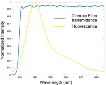
2.4 Fluorescence spectrum of cytometry bead and dichroic mirror transmission spectrum in TRACK cytometry experiments . . . 36

2.5 Target tracking by TRACK technique . . . 38

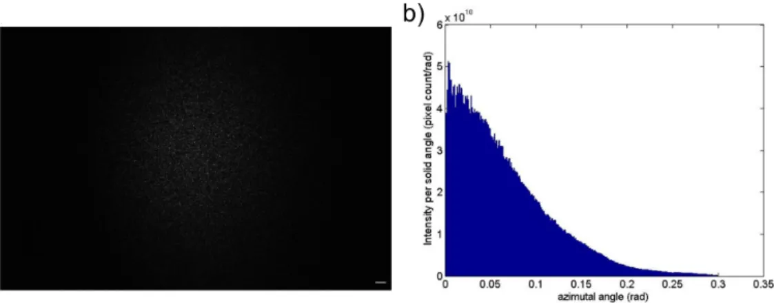
2.6 Optical flow cytometry in scattering media using TRACK technique . 39 2.7 TRACK focusing results through 0.5 mm thick chicken breast tissue . 42 2.8 Angle distribution of the diffusing sample used for TRACK experiments 43 2.9 Comparison between TRACK and traditional DOPC . . . 43

2.10 Timing for the TRACK experiments . . . 44

3.1 Simplified schematic of the DMD based DOPC . . . 50

3.2 Functional schematic of FPGA based DOPC. . . 52

3.3 DMD diffraction demonstration and binary phase modulation of DMD 53 3.4 Workflow of FPGA based DOPC. . . 56

3.5 Playback latency quantification . . . 57

3.6 DMD based DOPC system PBR quantification . . . 58

3.7 DMD based DOPCIn vivoexperimet setup and results . . . 59

(11)

3.8 Full setup diagram for DMD based DOPC system . . . 63

3.9 Relation between normalized theoretical PBR and the upper bound of the absolute phase difference in DMD based DOPC . . . 67

3.10 Single shot binary phase retrieval . . . 69

4.1 Principle of the CGN technique . . . 77

4.2 Experimental demonstration of CGN . . . 80

4.3 Characterization of glare suppression factor . . . 83

4.4 Reconstruction of the target at different distances using CGN . . . 84

4.5 Comparison of CGN and CG techniques . . . 85

4.6 Characterization of glare back-reflected from a scattering medium . . 88

4.7 Ideal glare suppression factor in different conditions computed via simulation. . . 89

4.8 Measured glare suppression factor in different conditions. . . 89

4.9 Schematic setup of Michelson interferometer for characterizing the coherence properties of the light source in CGN . . . 90

4.10 Light Source Coherence Characterization in CGN . . . 91

5.1 Principle behind non-invasive imaging of obscured moving objects . 97 5.2 Impact of object travel distance on the computed speckle autocorrelation (SAC) . . . 100

5.3 Experimental setup for imaging hidden moving objects . . . 102

5.4 Experimental imaging of moving targets hidden behind a diffuser . . 103

5.5 Experimental results showing the effect of object motion distance on the speckle autocorrelation (SAC) and object reconstruction . . . 104

5.6 Experimental retrieval of moving targets hidden within a scattering object . . . 106

(12)

C h a p t e r 1

INTRODUCTION

Focusing and imaging correspond to two basic requirements in utilizing light: ma- nipulating and observing. Optical focusing and imaging are of great importance in biomedicine, remote sensing, astronomy, industrial production, to name a few. The advantage of using light can be summarized in three aspects, as follows.

First, optical resolution is only limited by diffraction, and can reach sub-micrometer scale [1]. It enables optical focusing to have a precise spatial selectivity, which allows for stimulation or manipulation of micro structures and micro processes.

For example, photolithography [2, 3] is an indispensable tool for integrated circuit fabrication, and optical focusing is also widely used for the control of cellular or sub- cellular biological systems, such as in photodynamic therapy [4], photoreleasing [5], optogenetics [6, 7], and optical cell trapping and shearing [8, 9]. Optical imaging with its fine resolution opens a door to the microworld through direct visualization.

Optical microscopy [10, 11] has long been a reliable tool in diagnosis. Recent development in super-resolution microscopy [12–16] has pushed the resolution limit down to tens of nanometers, even several nanometers. Although electron [17]

and scanning probe microscopy [18, 19] inherently possess a finer resolution (sub- nanometer), optical microscopy is still the only way to observe living processes at micro scale without harsh preparation procedures.

Second, due to the physical interaction between light and matter, it is possible to use optical focusing and imaging to investigate material compositions through spectroscopy, polarization, photoluminescence, and photoacoustics [20]. For instance, Raman spectroscopy [21–24] is extensively used to observe vibrational, rotational, and other low-frequency modes in a molecular system.

Third, optical focusing and imaging have the ability to perform at high temporal resolution. It enables us to control and observe temporal evolution of physical events, which led to the advent of ultrafast optics [25]. Tremendous efforts have been made in the development of ultrafast spectroscopy [26, 27], laser-controlled chemistry, and so on, among which one exciting achievement is that the world’s fastest 2-D camera up to date can capture events at up to 100 billion frames per second [28].

(13)

Conventionally, optical focusing and imaging are realized by lenses in a transparent medium, like air or glass, which are based on the ballistic propagation of light.

However, when light propagates through most scattering media, refractive index inhomogeneities cause diffuse scattering that increases with depth. This poses a major challenge to all the aforementioned optical methods. Moreover, glare caused by backscattering will largely impair the visibility of imaging, and time-varying scattering by dynamic media will also pose a challenge to the system response time. All of these factors fundamentally limit the feasibility of optical focusing and imaging in scattering media, such as biological tissues and fog. In this chapter, we provide an overview of the physics behind optical scattering, discuss the challenges brought in, and introduce different methods used to overcome scattering.

1.1 Physics of Scattering

Light interacts with matter in many different ways including absorption, elastic scattering, inelastic scattering, quasi-elastic scattering, nonlinear process. Here we limit our discussion to elastic scattering, which causes light to diffusively propagate in scattering media. We will first start with single particle scattering model, and then expand our discussion to a group of particles. Finally, based on the model, we will discuss the properties of real scattering media and conclude with some general

"rules of thumb" that are useful when considering the interaction of light with tissue.

Scattering of a single particle

Figure 1.1: Rayleigh scattering and Mie scattering [29]

A simple model to start with is the scattering of a single small particle, which can be described as Rayleigh scattering or Mie scattering [30–32], as shown in Fig. 1.1.

For particles much smaller than the wavelength of the incident light, their scattering of light can be explained by Rayleigh scattering. It is an approximation derived from the interaction between light and a dipole. The scattered intensity distributionI(r, θ)

(14)

(expressed in polar coordinates) for unpolarized incident light can be expressed as [30, 32]

Is(r, θ) = 8π⁴nsu4( ns2−nsu2

ns2+2nsu2) a⁶

r²λ⁴(1+cos²θ)I₀, (1.1.1) where I₀ is the incident light intensity, λ is its wavelength, ns and nsu are the respective refractive indices of the scatterer and its surrounding medium, and a is the radius of the scatterer.

Mie scattering is applied when the particle size is on the order of the wavelength.

It can be derived by solving Maxwell’s equations for the case of a spherical scatter, composed of homogeneous and isotropic material, that is irradiated by a monochromatic plane wave [33]. The angular intensity distribution of scattered light for two perpendicular polarizations can be describe as,

I₁(θ)=

∞

X

n=1

2n+1

n(n+1)[anπn(cosθ)+bnτn(cosθ)]

2

, (1.1.2)

I₂(θ)=

∞

X

n=1

2n+1

n(n+1)[bnπn(cosθ)+anτn(cosθ)]

2

, (1.1.3)

whereanandbnare coefficients defined by the boundary conditions, andπn(cosθ) andτn(cosθ)are the Mie angular functions. The functions can be described as

πn(cosθ) = 1

sinθP_n¹(cosθ), (1.1.4) τn(cosθ) = d

dθP_n¹(cosθ), (1.1.5) where P_n¹are associated Legendre polynomials of the first kind. In both cases, we can conclude that incident beam is deflected from its original propagation. A narrow incident beam will be scattered into a cone of beams with different directions. Aside from forward scattering, there is backscattering as well.

Based on the single particle model, we can derive more parameters to characterize the scattering of light by a single particle. One important parameter is the scattering anisotropyg[32],

g=< cos(θ) > , (1.1.6)

where θ is the scattering angle. g describes the angular spread of light scattered off a particle. The values of g can range from -1 to 1, where a lower negative value indicates more backward scattering, while a higher positive value indicates more forward scattering. Another important parameter for a single scatterer is its

(15)

scattering cross sectionσs [mm²]. σs indicates the particle’s scattering capability.

It can be thought of as the effective area that guarantees scattering when a photon impinges. σs is related to its geometric cross-sectional area A [mm²] by the proportionality constant called the scattering efficiencyQs [dimensionless], which is described as σs = QsA. Note that Qs takes on a statistical nature and is not necessarily equal to the physical cross section area of the scatterer.

Scattering of a collection of particles

Based on the scattering model of a single scatterer, we expand our discussion to the scattering of a collection of homogeneous scatterers that are randomly distributed within a finite three-dimensional space. This is a simplified model of a real scattering medium. The scattering characteristics of the sample per unit length are described by the scattering coefficient µs [mm⁻¹] and the scattering mean free path (MFP)ls

[mm]:

µs = σsN, (1.1.7)

ls = 1 µs

, (1.1.8)

whereNis the number of scatterers per unit volume [mm⁻³]. The scattering MFP is the average distance between scattering events. Fromls, we can derive the intensity of ballistic light after light travels a thickness ofl through the sample [32],

Ib(l) = I₀e⁻^ls^l = I₀e^−µ^s^l. (1.1.9) Eq. 1.1.9 only quantifies how many photons are scattered. It doesn’t consider how much the photons have deviated from their original trajectory. For example, ifg ≈1 and a photon encounters many scattering events, the trajectory of the photon will still not deviate from its ballistic trajectory too much. In other words, the photon retains some "memory" of its original orientation. To eliminate this "memory", the anisotropy of the scatterers is incorporated to characterize the scattering sample by their reduced scattering coefficientµs0

[mm⁻¹] or transport mean free path (TMFP) ls0

[mm], which are defined as,

µs0= (1−g)µs, (1.1.10)

ls0= 1

µs0. (1.1.11)

From the equations, we can tell µs0

is a lumped property incorporating µs and g. By multiplying µs by a factor of (1− g), we convert the photon movement

(16)

with many small steps 1/µs that involve only partial deflection to a random walk of step size 1/µs0

. We can think of the TMFP as the mean distance after which a photon’s direction becomes randomized. By the definition of MFP and TMFP, people divide light propagation in scattering media into four different regimes [32, 34, 35]. Within one MFP through a scattering media, ballistic photons are still dominant. This regime is called ballistic regime. In the region from the MFP to the TMFP, photons are scattered a few times but are just slightly deflected from their paths. This regime is called the quasi-ballistic regime. Between one and ten TMFPs, incident photons have been scattered many times but still retain some "memory" of their original directionality. This regime is called quasi-diffusive regime. Finally, beyond ten TMFPs, the directions of the scattered photons are barely related to its original directions. This regime is called diffusive regime. If you want to directly visualize the difference of scattering in different regimes, please refer to a schematic depiction from Vasilis Ntziachristos’s paper [34].

The particle model described above is an inaccurate approximation for a real scattering medium. Consider the case of biological tissue for example. Its micro-structure is more complicated than smaller particles of the same identity suspended in a uniform environment. Biological tissues can have micro structures ranging from 0.01 µm for membranes to 10 µm for whole cells [32, 36]. The refractive indices of scatterers can also vary from 1.34-1.62 for different tissue components [32, 36].

Therefore, it is really difficult to solve the scattering of a real scattering medium through all the micro processes and then find a solution to counter its influence.

However, the model we use is accurate enough when considering the scattering process at the macro scale, such as in estimating the portion of ballistic transmission and randomness of transmitted wavefront. We may have a chance to draw some useful conclusions from the macro-phenomena of scattering and then come to some useful tools by either resolving or utilizing scattering. This leads to the discussions in the following sections.

1.2 Macro-Phenomena of Scattering Speckle

When a single optical mode is shone onto a scattering medium, light propagates diffusively within the scattering medium, as shown in Fig.1.2(a). The concept of optical mode will be discussed in the end of this section. For now, we can just take it as a beam that is perfectly monochromatic and as narrow as possible. After traveling beyond the diffusive regime, the output will be a spatially uncorrelated

(17)

Figure 1.2: Schematic depiction of light’s diffusive propagation and output wavefront through a scattering medium. (a) A perfectly monochromatic beam propagates through a scattering medium. (b) At an arbitrary point on the output wavefront, the electric field can be deemed as a summation of different beamlets.

wavefront. Initially, we limit attention to a single polarization state, since the same analysis will apply for the other polarization. At an arbitrary point A(x,y) on the output surface z = zout put, the output optical field is a summation of beamlets that encounter different scattering events, as shown in Fig. 1.2(b). Moreover, from the previous section we know that the scattering of each beamlet can be considered a random process. Thus, we can consider the output electric field of every beamlet at point A as a random variable ak(x,y) and the output electric field at point A, E(x,y) can be described as summation ofak(x,y) in the complex plane as shown in Fig. 1.2(b),

E(x,y)=

N

X

k=1

ak(x,y) =

N

X

k=1

|ak(x,y)|e^iθ^k, (1.2.1) where |ak(x,y)| and θk are the amplitude and phase of ak, respectively. If we decomposeE(x,y)into the real and imaginary parts, we have

E(x,y) =Re(E(x,y))+iIm(E(x,y)), (1.2.2) Re(E(x,y)) =

N

X

k=1

|ak(x,y)|cosθk, (1.2.3)

Im(E(x,y)) =

N

X

k=1

|ak(x,y)|sinθk. (1.2.4) We know that ak(x,y) is generated by the incident beam with limited energy, so

|ak(x,y)|should possess limited mean value and variance. Note that we have only shown fourak(x,y)s that sum up at point A in Fig. 1.2(b). In fact, N is very large, considering the fact of diffusive propagation of light in the medium. Therefore,

(18)

we can apply the central limit theorem to Eqs.1.2.3 and 1.2.4, which simply means Re(E(x,y,z))and Im(E(x,y))follow a Gaussian distribution. By evaluating their first-order statistical properties, we can find out that the real and imaginary parts of the output field have zeros means, identical variances, and are uncorrelated.

Supposing Re(E(x,y))follows a Gaussian distribution with zero mean and variance σ², the joint probability function of Re(E(x,y)) and Im(E(x,y))is

p(Re(E(x,y)),Im(E(x,y)))= 1

2πσ²exp −[Re(E(x,y))]²+[Im(E(x,y))]² 2σ²

! . (1.2.5) Such a density function is commonly known as a circular Gaussian density function.

Therefore,E(x,y)can be referred to as a circular complex Gaussian random variable.

For the output wavefront, it is more straightforward to talk about its amplitude

|E(x,y)|, intensityI(x,y), and phaseθ(x,y). We can apply the transformation of these random variables with reference to Re(E(x,y))and Im(E(x,y))as follows:

|E(x,y)|= q

[Re(E(x,y)]²+[Im(E(x,y)]², (1.2.6) I(x,y) = [Re(E(x,y)]²+[Im(E(x,y)]², (1.2.7) θ = Arg(Re(E(x,y))+iIm(E(x,y))). (1.2.8) Then the probability density functions of |E(x,y)|,I(x,y)andθ(x,y)are

p(|E(x,y)|) =













σ1²exp

−|E(x,y)|² 2σ²

,if|E(x,y)| ≥ 0

0 ,otherwise

, (1.2.9)

p(I(x,y)) = 







1 2σ² exp

_−I_(x,y)

2σ²

,if |I(x,y)| ≥ 0

0 ,otherwise

, (1.2.10)

and p(θ(x,y)) = 









1

2π ,if −π ≤ θ(x,y) < π 0 ,otherwise

. (1.2.11)

From the equations, we can conclude that the intensity of the output wavefront follows a negative exponential distribution, the amplitude follows a Rayleigh distribution, and the phase possesses a uniform distribution [37]. The phase and amplitude are independent. The statistics have been confirmed in experiment. Fig. 1.3(a) is an intensity pattern of a scattered wavefront we captured by a CCD sensor with an objective lens. We can tell the two-dimensional intensity distribution is a speckle pattern. A two-dimensional histogram of the amplitude and phase of speckle pattern is shown in Fig. 1.3(b), which matches the probability distribution of phase

(19)

and amplitude. Note that speckle is the smallest feature in a speckle pattern. The speckle size is defined by the diffraction limit _{N A}^λ , where the numerical apertureNA is the sine of the maximum take-off angle of light on the output surface. By the Shannon’s sampling theorem, within the half width of a speckle₂_{N A}^λ , the amplitude and phase can be deemed as uniform. An area of ( ^λ

2N A)²on the output surface can be treated as a single optical mode. This clarifies the definition of an optical mode at the beginning of this section. This is also why we can discretize a continuous wavefront into an array of discrete optical modes, which we will frequently use in the transmission matrix theory. A rigorous proof of wavefront discretization can be found in the supplementary material of reference [38].

Figure 1.3: Statistics of the output scattering wavefront. (a) The spatial intensity pattern of the output scattering wavefront. (b) 2D histogram of the phase and amplitude of the output scattering wavefront.

The previous discussion was based on a single mode input. If we have a wide incident beam or multiple input modes, the conclusions still hold. Without loss of generality, let’s suppose we have two input modes, their output wavefronts are E₁(x,y) and E₂(x,y). Re(E₁(x,y)) and Im(E₁(x,y)) follow a Gaussian distribution with zero mean and variance σ₁², while Re(E₂(x,y)) and Im(E₂(x,y)) follow a Gaussian distribution with zero mean and variance σ₂². If the incident beams are perfectly monochromatic, the output wavefront will be a coherent summation ofE₁(x,y)and E₂(x,y). That is Eout put(x,y) = E₁(x,y)+ E₂(x,y). If E₁(x,y) and E₂(x,y) are independent, Re(Eout put(x,y)) follows a Gaussian distribution with zero mean and varianceσ₁²+σ₂²by calculating the probability density function of summation of independent random variables, as does Im(Eout put(x,y)). Going through the same derivation as the case of a single incident mode, we come to the same statistical properties for output wavefront from multiple input modes.

(20)

Transmission matrix theory

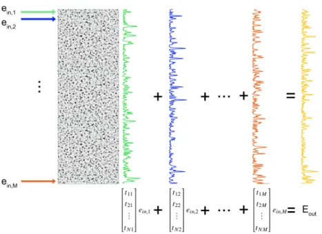
Figure 1.4: The output of a incident input wavefront can be deemed as the summation of the output wavefronts of every single input mode, as discussed in the previous section. The conclusion can also be expressed by the transmission matrix theorem as shown in Eq. 1.2.14.

If we treat the process through which light propagates inside the scattering media as a linear lossless process of the optical field and look at the input and output wavefronts, we can describe scattering as a linear transform between the two [39–

41]. Based on the discussion in the speckle section, the input and output wavefronts can be discretized as elementwise arrays of optical modes. Suppose array Ein and array Eout represent the input and output wavefront and have M and N elements, respectively. Every element ofEinandEoutis the complex value of the corresponding optical mode. The transform can be represented by a N by M transmission matrix Tin→out, which describes how the phase and amplitude of the input field is modified by the medium and presented on the output plane. Its mathematical representation is [40]

Eout =Tin→outEin. (1.2.12)

(21)

To be more clear, an elementwise expression of Eq. 1.2.12 is







t₁₁ t₁₂ . . . t₁M

t₂₁ t₂₂ . . . t₂M

... ... ... ...

tN1 tN2 . . . tN M











 ein,1

ein,2

...

ein,M







=







t₁₁ein,1+t₁₂ein,2+· · ·+t₁Mein,M

t₂₁ein,1+t₂₂ein,2+· · ·+t₂Mein,M

...

tN1ein,1+tN2ein,2+· · ·+tN Mein,M







=





 eout,1

eout,2

...

eout,N





 ,

(1.2.13) wheree_in,k ande_out,k are thekth element in arrayEin andEout, respectively andti j

is the element at theith row and jth column of the transmission matrixTin→out. If we take a close look at the terms on the left and right of the second equal sign in Eq. 1.2.13, we can rewrite the equation as

Eout =











 t₁₁ t₂₁ ...

tN1





 ein,1+





 t₁₂ t₂₂ ...

tN2







ein,2+· · ·+





 t₁M

t₂M

...

tN M





 ein,M







, (1.2.14)

which simply means that the output optical field is the summation of every individual output of a single input optical mode. A schematic demonstration is shown Fig. 1.4.

In the previous section, we derived the statistics of the output wavefront of a single input mode. In transmission matrix theorem, for a defined input modeein,j, its output wavefront is described as an array [t₁je_in,j,t₂pe_in,j, . . . ,tN je_in,j]. So that, t_k,je_in,j

should follow the circular Gaussian distribution due to its statistical property. For a definite j, ein,j is a complex constant, so it isti j that possess a circular Gaussian distribution. In other words, every element in the same column of the transmission matrix follows a circular Gaussian distribution. If every column of the transmission matrix is independent, then every element ti j in the transmission matrix Tin→out

follows a circular Gaussian distribution. Generating a random matrix with circular Gaussian distributed elements is usually how people simulate a scattering medium.

Transmission matrix theory is widely used in the analysis of wavefront shaping and phase conjugation. We will see more derivations based on this in the following sections.

Memory effect

In the previous section, we modeled the scattering as a transmission matrix. For a real scattering medium, its transmission matrix can have an additional macroscopic structure, either correlation in spatial domain or Fourier domain, depending on its scattering property. Memory effect is the manifestation of correlations in the

(22)

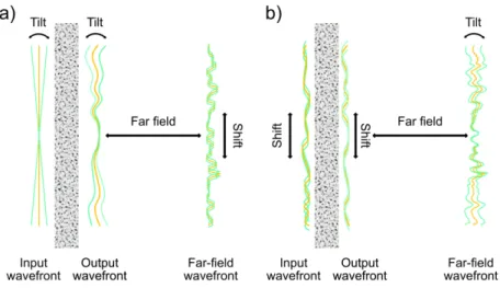
Figure 1.5: Schematic depiction of two types of memory effects. (a) Traditional memory effect. (b) Translational memory effect.

transmission matrix. Up to date, two types of memory effects have been discovered.

They are the traditional memory effect [42, 43] and the translational memory effect [38], respectively.

The traditional memory effect for a general scalar wave was first derived theoretically in 1988 [42]. It was verified experimentally for optical waves in the same year [43].

The traditional memory effect describes the following phenomenon: when an input wavefront reaching a diffusing sample is titled within a certain angular range, the output wavefront is equally tilted, resulting in a spatial shift of the speckle pattern at far filed, as shown in Fig 1.5(a). The distance within which this property holds is called the memory effect region (MER). It can be approximated by the equation [38],

MER≈ vλ

πL, (1.2.15)

wherevis the distance from the output plane of the scattering medium to the screen, λ is the wavelength of the light source and L is the thickness of the scattering medium. From the equation, the MER is inversely proportional to the thickness of the scattering media. For useful applications, it requires the scattering medium to be thin. Moreover, it requires a distance of far-field propagation to realize the shift of the output wavefront. The conjugate planes of the tilt-and-shift relation is the input surface and the far-field plane. If we think inversely of the phenomenon, a point source within the MER will generate a random speckle pattern through the scattering medium. When we shift the point source, the speckle pattern will also

(23)

shift at far field. If we treat the speckle pattern as a point spread function (PSF), the PSF will be shift-invariant within the MER, which is similar to the scenario in a traditional lens based imaging system. People have demonstrated direct image transfer and computational image recovery based on the traditional memory effect.

We will see some related work we have done in Chapter 5.

The translational memory effect was first reported in 2015 [38]. It is a complemen- tary type of memory effect to the traditional one. It describes the following phenomenon: when an input wavefront reaching an anisotropically scattering medium is shifted within a certain distance, the output wavefront is equally shifted, resulting in the tilting of far-filed wavefront, as shown in Fig. 1.5(b). The translational memory effect applies for thick and highly forward scattering media, such as biological samples. Different from the traditional memory effect, its shift-invariant PSF region is on the output surface the scattering medium, which has important implication for biomedical imaging and adaptive optics.

There are also many other macro-phenomena discovered on optical scattering, such as the shower-curtain effect [44–46] and Anderson localization [47–49]. We will not talk about them in detail.

1.3 The Problem of Scattering

As briefly discussed in the abstract, scattering is a major challenge for optical focusing and imaging. In this section, we will analyze three effects that hinder optical focusing and imaging through scattering media, which are wavefront aberrations, glare, and decorrelation.

Wavefront aberration

Wavefront aberrations originate from the diffusive propagation of forward-scattering light through scattering media. They are the differences between the scattered wavefront and the wavefront intended to present through a scattering medium. Wavefront aberrations induced by scattering are different from the wavefront aberration in a lens system [50, 51]. First, it cannot be predicted by the geometrical setup such as aperture size, propagation distance, and lens shape [52]. Second, the order of scattering wavefront aberration is very high, considering the fact that the output wavefront is made up of diffraction limited speckles. As such, the aberrations cannot be compensated by traditional lens design. As shown in Fig. 1.6(a), a collimated beam is focused on the focal plane by a lens in free space. However, if we applied the same strategy in the presence of a scattering medium, the outcome will be a speckle

(24)

Figure 1.6: Schematic depiction of problem of scattering for focusing light through a scattering medium. (a) Optical focusing can be easily realized by a lens in free space. (b) Scattering media leads to a diffusive propagation, which results in a random output wavefront.

field on the focal plane. Based on the statistical property of speckle pattern, light intensity is not well confined to a small region so that it lost its spatial selectivity.

For imaging, conventional imaging systems relies on lenses and mirrors to transform light from a point on the object plane to a point on the image plane [53, 54]. If there is a scattering medium in front of the object, the PSF will spread out as a speckle field. The point-to-point conjugate relationship between the object and image is broken by the wavefront aberrations. Therefore, conventional optical methods will fail when they are applied to imaging through scattering media.

Glare

Figure 1.7: Experimental demonstration of issue brought by glare. (a) shows the captured camera image with a reflective illumination. The glare from the light source prevents us from seeing the target. (b) shows a captured image where the figurine is locally illuminated.

Glare is the undesired backward-scattering light when we illuminate a scattering

(25)

sample [55, 56]. It impacts imaging more than focusing. When we try to image a target through a scattering medium, in most cases such as remote imaging in fog, haze, and sandstorm, we don’t have access to the other side of the scattering media.

Therefore, a reflective illumination setup has to be adopted over trans-illumination, which means the light source and the detector are on the same side with reference to the sample. In the reflective illumination scenario, light first propagates through the scattering medium before illuminating the target. The glare from the illumination source impinging on the scattering medium can mask the reflections from a weak distant target [57–59]. An experimental demonstration is shown in Fig. 1.7. This brief experiment illustrates the issue: glare can significantly reduce our ability to image or probe into scattering media. Here we point both a camera and a spotlight at a fog bank (generated by a fog machine). A figurine is on the other side of this fog bank. Fig. 1.7(a) shows the captured camera image with the spotlight illumination.

The glare from the spotlight prevents us from seeing the figurine. Fig. 1.7(b) shows a captured image where the figurine is locally illuminated. Despite the slight blurring introduced by scattering from the fog, we can readily discern the figurine.

The more challenging part is that the glare wavefront generated by a coherent light source is a speckle field with severe intensity variance. Even if an incoherent light source is used, the glare will still show up as an uneven noise term, as we can see from Fig. 1.7(a). Moreover, if the glare intensity is too high, its shot noise will overwhelm the signal. Glare as a strong background cannot be easily removed by simple digital signal processing such as background subtraction and contrast enhancement. Physical methods are required to suppress the glare or separate it from the target reflection.

Decorrelation

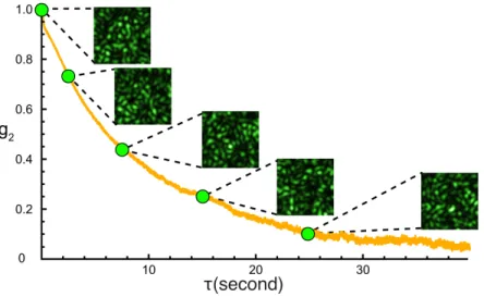
All the previous discussion is based on a static scattering media. However, many scattering media we frequently deal with are dynamic, whose micro structure or composition is changing over time. For example, living biological tissues can have blood cells moving continuously in the vessel. The refractive indices of cytoplasm in cells will also vary based on metabolism. Fog is made up of small droplets of water in the condensed phase. The water droplets are kept in the air by thermal Brownian motion. All of these micro changes will accumulate and lead to a time-varying output wavefront when we shine a coherent beam through the sample[60–63]. The change of the output wavefront can be described as a decorrelation process and characterized by its intensity autocorrelation function based on the diffusing-wave

(26)

spectroscopy [64]. Suppose the mean intensities of speckle patterns at different times are the same, then the autocorrelation function can be written as [65, 66]

g₂(τ) = < I(x,y,t₀)I(x,y,t₀+τ) >x,y

< I(x,y) >_x,y² −1, (1.3.1) where< >_x,_y represents the ensemble-average in the capture plane, I(x,y,t)is the speckle pattern at timet, and τis the time interval. According to the assumption,

< I(x,y) >x,y=< I(x,y,t₀)x,y >=< I(x,y,t₀+ τ)x,y >. g₂(τ) is the correlation factor. From the statistics of speckle, we know that g₂(τ) can range from 0 to 1,

Figure 1.8: Measured decorrelation curve of a 1 mm thick rat brain tissue.

which corresponds the change of correlation. Then the speed of decorrelation can be describe as ∆g₂/τ. However, as shown in Fig. 1.8, the decorrelation process doesn’t always follow a linear fashion. Fig.1.8 is an example of a decorrelation curve measured in experiment. Therefore, decorrelation time is more commonly used to describe how fast a tissue decorrelates. It is the time intervalτafter which theg₂(τ)autocorrelation factor decays to a pre-determined value, typically 1/e², 1/e [66–71]. If we choose 1/e²as a standard, for example, the decorrelation time τ₁_/e2

for the dorsal skin of a living mouse with 1.5 mm thickness can be shorter than 50 ms [66, 69].

Decorrelation poses a challenge for the techniques that work under the assumption that scattering is static. For example, wavefront shaping technique is a novel technique that can focus light through scattering media, which we are going to introduce in the following section. However, decorrelation will disrupt the focus by changing the transmission matrix [66]. The general solution is to speed up the system and

(27)

keep its response time shorter than the decorrelation time, which we will discuss detailedly in Chapter 3.

1.4 Methods for Optical Focusing and Imaging through Scattering Media In this section, we will give a brief review on the techniques to realize optical focusing and imaging through scattering media. The discussion will focus on the concepts and principles. First, we will talk about wavefront shaping, a novel method that enables optical focusing through scattering media. Then, we will go through different methods people use to realize imaging through scattering media. Finally, we will introduce techniques for glare suppression.

Wavefront shaping

Although focusing through scattering media has long been considered impossible, recent developments in wavefront shaping (WFS) have changed this view. The basic principle behind WFS is rooted in the transmission matrix theory. Let’s first take a back look on Eq. 1.2.14:





 eout,1

eout,2

...

eout,N







=











 t₁₁ t₂₁ ...

tN1





 ein,1+





 t₁₂ t₂₂ ...

tN2







ein,2+· · ·+





 t₁M

t₂M

...

tN M





 ein,M





 .

For a single output modeeout,1, we have

eout,1 =t₁₁ein,1+t₁₂ein,2+· · ·+t₁Mein,M =

N

X

k=1

t₁kein,k. (1.4.1) When the input is a plane wave, e_in,k is identical for k ∈ [1,M]. t₁ke_in,k is out of phase for different k, resulting ineout,1as a speckle. If we can control the phase of ein,k and set arg(ein,k) = −arg(t₁k), we can linet₁kein,ks up in the complex plane, as shown in Fig. 1.9(b). Lete⁰_out,

1be the output after we optimize the phase of each input mode, then|e⁰_out,

1|can be expressed as

|e⁰_out,

1|=

N

X

k=1

|t₁k|eârg^(t¹^k⁾|e_in,k|eârg^(eîn,k⁾

=

M

X

k=1

|t₁k||e_in,k|. (1.4.2)

Comparing to its modulus before the optimization,|e_out,₁|, which is

|eout,1|= |

M

X

k=1

t₁kein,k|, (1.4.3)

(28)

we can derive the intensity enhancement factorηas η = < |e⁰_out,

1|² >

< |eout,1|² > =

PM

k=1|t₁k||ein,k|

2 D|PM

k=1t₁kein,k|²E =

PM k=1|t₁k|

2 D|PM

k=1t₁k|²E. (1.4.4) Then we try to figure out the intensity of unoptimized modes (the background), it can be proved that their mean intensity before and after optimization are nearly the same, when M is much greater than N [35, 40]. < |e_out,₁|² > is equal to the background before optimization, so < |e_out,₁|² > can approximate the background after optimization as well. Therefore,ηis also the signal to background ratio or peak to background ratio (PBR) after WFS. From the statistics of a transmission matrix,

Figure 1.9: Schematic depiction of different modulation strategies. (a) Original unmodulated phasors out of phase. (b) Phase modulation. (c) Binary phase modulation. (d) Binary amplitude modulation.

we know thatt₁k follows circular Gaussian distribution, then we can findη = ^π₄M. If we want to enhance the intensity in multiple output modes, going through the same calculation, we find that η = ^π₄^M_N, where N is the number output modes to optimize. If we "shape" the input wavefront, we can focus light to a small region through scattering media.

The modulation of input modes can be relaxed to binary phase modulation or binary amplitude modulation in different experimental scenarios, which will still lead to an enhancement in the target output modes as shown in Fig.1.9(c) and (d). Fig.1.9(c) depicts the method by which binary phase modulation enhances the target output mode. If we shift the phase of phasor 2 and 3 byπ, then all the output modes are partially lined up. In contrast, for binary amplitude modulation, we switch off all the input modes that negatively contribute to the the target output mode intensity.

As shown in in Fig. 1.9(d), we turned off phasor 2 and 3 and only used phasor 1 and 4. Going through the same calculation of enhancement factor as in Eq. 1.4.4, we

(29)

can summarizeηfor different modulation strategies as follows:

ηphase modulation = π 4

M N, ηbinaryphase = 1

π M N, ηbinaryamplitude = 1

2π M N,

(1.4.5)

where M is the number of controllable input modes, and N is the number of output modes to optimize. Chapter 3 is an example of application of binary amplitude modulation, a more detailed discussion on this strategy can be found in the principle section.

Thanks to the development of modern electronics technology, a spatial light modulator (SLM) can be used to shape the wavefront in practice. An SLM could be either a LCOS-SLM (liquid crystal on silicon-Spatial Light Modulator), a ferroelectric LC-SLM (liquid crystal-spatial light modulator) or a DMD (digital micromirror device), which can realize phase modulation, binary phase modulation or binary amplitude modulation, respectively. Then the question comes to how to find out the correct input wavefront. In general, the correct wavefront can be obtained by iterative optimization [72–80], measuring the transmission matrix [81–85] or by phase conjugation [86–95]. Iterative optimization requires a feedback signal that quantifies how much intensity is focused on the target modes. The feedback signal can be fluorescent light from a probe particle [72–74], photoacoustic wave [75, 76], ultrasound [77], second-harmonic generation [78], two-photon or multi-photon excitation [79, 80] or light intensity in the corresponding modes measured by a photodetector [40]. Iterative methods inherently suffers from a relatively long time of convergence, since the solution is found through trial and error. Transmission matrix measurement [81–85] can be deemed as an extension of iteration optimization. It is equivalent to figuring out the optimum input wavefront to all the output modes of interest. Transmission matrix measurement figures out the transmission matrix by measuring the output wavefronts with the pre-knowledge of corresponding input wavefronts. We can expect that transmission matrix measurement is even more time-consuming than iterative optimization. Moreover, in most situations of application, it requires direct access to the output plane.

Phase conjugation will be detailedly discussed in chapter 2 and 3. Here, we just give a brief introduction to the principle. Phase conjugation describes the reciprocity of light propagation in a linear and lossless medium [96, 97]: the phase conjugate

(30)

Figure 1.10: Schematic depiction of phase conjugation

reflection of a wavefront is a "time-reversed" replica of the wavefront’s electric field.

As shown in Fig.1.10, if we place a point source at the target mode, then light will propagate through the scattering medium and generate an output wavefront. At the output plane, if the wavefront is reflected off the output plane with a conjugate phase, scattered light will retrace their propagation and result in light focusing back at the target mode, as if time is reversed. From the process of phase conjugation, we know that, if we can have a focus at the target mode, the correct input wavefront for WFS can be easily figured out by measuring the wavefront coming out of the scattering media and conjugating the measured phase. However, the requirement to originally have a focus at the target mode where we aim to focus defeats the purpose of WFS. A way around this problem is to phase conjugate light from a guide star [98]. A guide star could be a small fluorescent particle [88] or a second harmonic generating particle [86] embedded in the scattering media. An alternative approach is to use ultrasound tagging to create a virtual guide star [67, 87, 89]. However, these guide stars all have their limits and disadvantages in application. For example, it is difficult to place small particles to a designated position without direct access to the target plane. For ultrasound tagging, the tagged photons are only a small portion compared to the total number of photons sent in, which may lead to a small signal to background ratio in the captured wavefront. Therefore, more noninvasive guide stars with better control and higher efficiency are still waiting to be discovered.

(31)

Methods for imaging through scattering media

Generally speaking, three approaches can be used to realize imaging through scattering media in the diffusive regime. The first is to scan the focus obtained by WFS.

From the discussion in the previous section, we know a tight focus can be formed through scattering media by WFS. If the WFS technique used, like TRUE technique [67, 87], has ability to select an arbitrary mode through the scattering media, then we are able to scan the focus over the object. Scanning can also be realized with the assistant of memory effect [99], but it has limitation in the thickness of the scattering media and scanning range. Moreover, the object has to be placed at a distance behind the scattering media. Focus scanning approaches also require the signal generated by the object to be distinguished by the detector from the input light. Therefore, existing demonstration is limited to a fluorescent [67] or second harmonic generating [99] object.

The second approach is measuring the transmission matrix [81, 100]. As aforementioned in the transmission matrix section, transmission matrix describes the transform between input wavefront and output wavefront. In an imaging scenario, the input wavefront is the optical field to be found from the object, while output wavefront can be obtained from measurement. If we know the transmission matrix, then the object can be figured out by solving the inverse problem of the transform.

As discussed in the WFS section, it is difficult to acquire the pre-knowledge of transmission matrix without access to the object plane. This approach shares the same limit with transmission matrix measurement in WFS. The third approach is the speckle-correlation-based imaging (SCI) [79, 101, 102], which we will discuss in detail in chapter 5. In general, optical imaging through scattering media still has a long way to go for application.

Methods for glare suppression

The optical field associated with glare and the reflected optical field from a remote target is different in an important way. Specifically, the glare components generally have a shorter optical path from source to detector. In principle, glare suppression can be performed using time-of-flight (TOF) methods [103–106] with the help of fast imaging systems, such as intensified charge-coupled device (ICCD) [107]. A TOF method would discard glare photons by binning the arriving light based on arrival time. Unfortunately, the requisite devices are very costly and, worse, tend to have very finite operating lifetime. There are some interesting developments in the use of modulated illumination and post-detection processing to achieve TOF

(32)

gating electronically [108]. One limitation for these methods is that they need to contend with glare associated noise, as the glare is not suppression prior to detection. Methods such as light detection and ranging (LIDAR) [109] can detect targets occluded by glare by coherently gated (CG) detection of light that have travelled a specific path length (or path length range). CG methods have a target range limitation—targets beyond the coherence length of the light source cannot be detected [110]. You will find more discussions on various glare suppression techniques in chapter 5. In general, there is not a comprehensive solution for glare suppression, as you can feel on the road when driving in a foggy day.

1.5 Outline of This Thesis

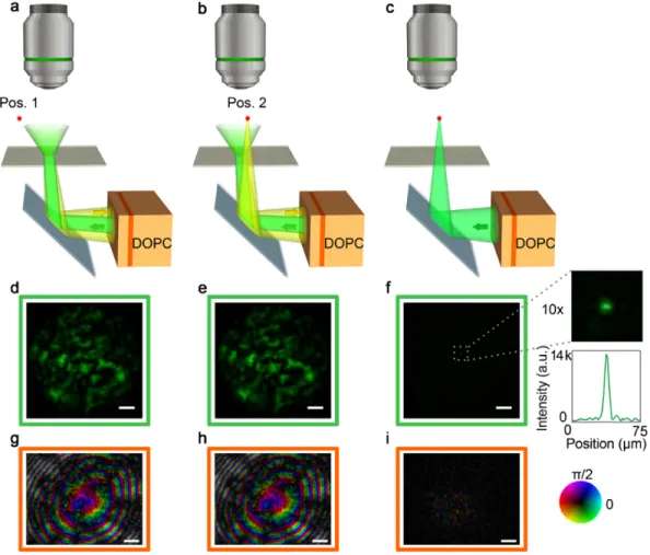
In this thesis, we will explore solutions to the problem of scattering from different aspects. Chapter 2 and 3 will aim on optical focusing through scattering media, while chapter 4 and 5 aim on imaging. Chapter 2 talks about Time Reversal by Analysis of Changing wavefronts from Kinetic targets (TRACK) technique. We will show that the motion of object can be incorporated as a guide star in phase conjugation.

We will demonstrate that by taking the difference between time-varying scattering fields caused by a moving object and applying optical phase conjugation, light can be focused back to the location previously occupied by the object. Chapter 3 tackles the decorrelation problem in wavefront shaping. We will talk about our strategies to speed up a DOPC system and demonstrate that our system is fast enough to focus light through 2.3mm-thick living mouse skin, which has a potential to transfer wavefront shaping toin vivoapplications. Chapter 4 introduces a glare suppression method based on destructive interference. We will show an optical analogue to noise canceling headphones and some experimental results in imaging through strongly backscattering media. Finally, in chapter 5, we will demonstrate a method to image a moving target through scattering media noninvasively. Its principle roots are in the speckle-correlation-based imaging (SCI) invented by Ori Katz. We will talk about how we improved the technique and extended its application to a bright field imaging scenario.

(33)

References

[1] Max Born and Emil Wolf. Principles of optics: electromagnetic theory of propagation, interference and diffraction of light. Elsevier, 1980.

[2] BJ Lin. Optical methods for fine line lithography. Elsevier, North Holland, 1980.

[3] Marc D Levenson, NS Viswanathan, and Robert A Simpson. “Improving resolution in photolithography with a phase-shifting mask”. In:IEEE Trans- actions on electron devices29.12 (1982), pp. 1828–1836.

[4] Thomas J Dougherty et al. “Photodynamic therapy”. In: Journal of the National Cancer Institute90.12 (1998), pp. 889–905.

[5] Graham CR Ellis-Davies. “Caged compounds: photorelease technology for control of cellular chemistry and physiology”. In:Nature methods4.8 (2007), pp. 619–628.

[6] Karl Deisseroth. “Optogenetics”. In:Nature methods8.1 (2011), pp. 26–29.

[7] Ofer Yizhar et al. “Optogenetics in neural systems”. In:Neuron71.1 (2011), pp. 9–34.

[8] Sylvie Hénon et al. “A new determination of the shear modulus of the human erythrocyte membrane using optical tweezers”. In:Biophysical journal76.2 (1999), pp. 1145–1151.

[9] JP Mills et al. “Nonlinear elastic and viscoelastic deformation of the human red blood cell with optical tweezers”. In:MCB-TECH SCIENCE PRESS-1 (2004), pp. 169–180.

[10] Mark C Pierce, David J Javier, and Rebecca Richards-Kortum. “Optical contrast agents and imaging systems for detection and diagnosis of cancer”.

In:International journal of cancer123.9 (2008), pp. 1979–1990.

[11] Jerome Mertz.Introduction to optical microscopy. Vol. 138. CSIRO, 2010.

[12] Stefan W Hell and Jan Wichmann. “Breaking the diffraction resolution limit by stimulated emission: stimulated-emission-depletion fluorescence microscopy”. In:Optics letters19.11 (1994), pp. 780–782.

[13] Mats GL Gustafsson. “Nonlinear structured-illumination microscopy: wide- field fluorescence imaging with theoretically unlimited resolution”. In:Pro- ceedings of the National Academy of Sciences of the United States of America 102.37 (2005), pp. 13081–13086.

[14] Michael J Rust, Mark Bates, and Xiaowei Zhuang. “Sub-diffraction-limit imaging by stochastic optical reconstruction microscopy (STORM)”. In:

Nature methods3.10 (2006), pp. 793–796.

[15] Eric Betzig et al. “Imaging intracellular fluorescent proteins at nanometer resolution”. In:Science313.5793 (2006), pp. 1642–1645.