The aim of the thesis is to develop the theoretical bases of optimization and generalization of learning in artificial neural networks. This chapter presents the central goal of the thesis: to find the foundations of optimization and generalization in artificial neural networks.
Optimisation via perturbation
The chapter develops a new technique called functional maximization that is essentially a perturbation analysis of the loss function operating on the function space of the machine learning model. They can be substituted into the functional size of the loss function to obtain new architecture-aware optimization methods for deep neural networks.
Generalisation via aggregation
Usually, in practice, one is interested in the generalization performance of only a single function—the one returned by the learning algorithm. In the case of hidden linearity (Equation 9.5), the approximation is correct when more than half of the ensemble agrees with the center of mass on an input.
Constructing Spaces of Functions
Kernel methods
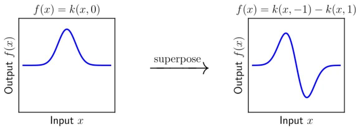
By superimposing kernel basis functions in this way, any kernel k(·,·) can be used to construct a space of functions. Furthermore, Equation 2.7 shows that the kernel interpolator of minimum RKHS norm can be represented using only finitely many kernel basis functions.
Gaussian processes
An advantage of this approach is that, given the training data, a posterior distribution over functions consistent with the data can be constructed simply by turning the handle of Bayes' rule. The next section will discuss how a posterior distribution can be constructed from the Gaussian process prior given data.
Neural networks
In words: the majorization hψ of convex functionψ is also assumed to majorize the loss function L. The reason this assumption is interesting is that the corresponding majorize-minimize algorithm has a particularly elegant form:. For a collection of m entries X ∈ Xm, let Xc denote all entries except X: Xc:=X \X. The result follows by substituting the chain rule for joint probability in the definition of the KL divergence, separating the logarithm and recognizing the two KL divergences:.
Correspondences Between Function Spaces
GP posterior mean is a kernel interpolator
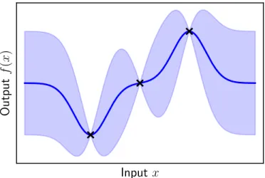
In these situations it may be sufficient to simply represent the mean of the posterior distribution (solid blue line in Figure 2.2). Perhaps surprisingly, the mean of a posterior distribution of a Gaussian process is equivalent to the kernel interpolator of the minimum RKHS standard, with the kernel set to the covariance function of the Gaussian process.
GP posterior variance bounds the error of kernel interpolation
But by Theorem 2.1 it is equivalent to the minimum RKHS norm kernel interpolator of (X, Y) with kernel k. In other words: if one approximates an unknown function g by the minimum RKHS norm interpolator f.
Making the GP posterior concentrate on a kernel interpolator
This foreshadows a contribution from Chapter 9, where a formal connection is made between Theorem 3.2 and a notion of normalized margin in neural networks. This formal connection exploits a correspondence between neural networks and Gaussian processes, which is presented in the next section.
Neural network–Gaussian process correspondence
For each input x∈Rd0, the components of the layer output fl(x) for that input are iid with finite first and second moments. The essence of this Gaussian process depends on the specific architecture of the network preceding the lth layer. But in this chapter the loss function will be considered as a simple function of the weights - formally, the loss L:W →R.
Perturbation analysis: Expansions and bounds
Majorise-minimise
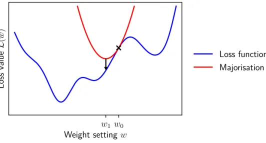
The core issue highlighted in the previous paragraph is that minimizing a truncated series expansion can lead to perturbations that are so large that the truncation is no longer a good approximation to the original loss function. 4.8) Taken together, these two conditions imply that a majorization provides an upper bound on the perturbed lossL(w+ ∆w) (Inequality 4.7) corresponding to the lossLat weight settingw. Since the majorization is both an upper bound on the loss that is also tangent to atw0, reducing the majorization to obtain a new weighting w1 also reduces the original loss.
Instantiations of the meta-algorithm
Finally, the following theorem shows that the gradient descent optimization algorithm emerges from the minimization of the principal in Inequality 4.10. The previous subsection showed that gradient descent in its most basic form arises from an intrinsically Euclidean majorization of the loss. Newton's method attempts to minimize the Taylor series expansion of the loss function truncated to second order:.
Trade-off between computation and fidelity
This chapter introduces two new techniques for machine learning optimization problems: functional majorization of the loss function and architectural perturbation bounds for machine learning models. Replace the architectural perturbation bounds with the loss functional maximization and minimize with respect to the weight perturbation to obtain an optimization algorithm. An odd aspect of this update is that the scale of the gradient only comes in logarithmically through η.
Majorise-Minimise for Learning Problems
Expanding the loss as a series in functional perturbations
The key idea is to Taylor expand the loss function in functional perturbations and then transform the linear terms in this expansion back into weight space. This extension is based on the fact that the machine learning loss function L can be thought of as a function of the weight vector w or a projected function fX(w) (Definition 2.1). The requirement from Lemma 5.1 that the loss function is analytic in the projection of the function space fX is mild.
Functional majorisation of square loss
The most common loss functions—including the squared loss (Definition 2.14) and the logistic loss (Definition 2.15) satisfy this requirement—. While the actual data discrepancy is usually easy to calculate or estimate in a machine learning problem, the latter two quantities are significantly more subtle.
First application: Deriving gradient descent
Second application: Deriving the Gauss-Newton method
Given a kernel k and a training sample S = (X, Y), we recall the definitions of the complexity of the kernel A (Definition 8.5) and the probability of the Gaussian orthant PY (Definition 8.4). These results will be used in Chapter 9 to study generalization in neural networks through the lens of the correspondence between the neural network and the Gaussian process. Given a kernel k and a training sample S = (X, Y), we recall the definitions of the complexity of the kernel A (Definition 8.5) and the probability of the Gaussian orthant PY (Definition 8.4).
Majorise-Minimise for Deep Networks
The deep linear network
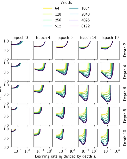
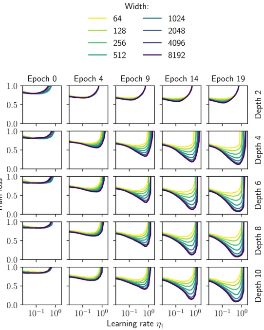
Although architectural perturbation bounds have been obtained for more general nonlinearities (Bernstein et al., 2020), the results obtained for deep linear networks in this chapter were already found to transfer experimentally to deep relu networks (Figure 6.1). It is important to note that the optimization landscape of the deep linear network is still non-convex due to the product of the weight matrices.
Architectural perturbation bounds for deep linear networks
Majorise-minimise for deep linear networks
Another feature of Update 6.11 is the clear dependence on both the network depth L and the scale of the kWlk weight matrices. On the other hand, equation 6.13 states that the operator norm and the Frobenius norm of the gradient ∇WlL(w) in layer l are equal. With equation 6.14, this occurs when ∇WlL(w) has only a singular nonzero value—meaning that the gradient is of very low order.
Experimental tests with relu networks
This thesis proves a new relationship, analogous to Lemma 9.1, between the BPM error and the Gibbs error. So the BPM approximation error ∆ measures the extent to which the BPM classifier and the Bayesian classifier disagree. Let αGibbs denote the average Gibbs consensus (Lemma 9.2) and ∆ denote the approximation error of the BPM.
Classic Generalisation Theories
Uniform convergence
The mechanism for proving uniform convergence bounds relies on the size of a function space being, in a sense, small compared to the number of training examples. In the case of binary classification, a convenient means of counting functions is to count the number of distinct binary labels that the function space is able to assign to a finite set of inputs. Provided that the refractive index saturates in a number of training examples m, then the bound is O(1/√m).
Algorithmic stability
Neural networks often operate in a regime where they can realize essentially any labeling of their training set (Zhang et al., 2017). It is not obvious whether neural networks satisfy a stability condition such as Definition 7.3 at the non-trivial level β. Sometimes neural networks are seemingly able to interpolate any training set (Zhang et al., 2017), meaning they are very sensitive to the inclusion or exclusion of any particular data point.
PAC-Bayes
In words, for linear classifiers, the BPM classifier is equivalent to a single point in weight space: the center of mass of the posterior Q. Thus, under the stated conditions of Lemma 9.4, the BPM error cannot exceed e times the Gibbs error . But if the BPM approach (Approach 9.4) is good, then the BPM classifier should inherit the same favorable properties as the Bayesian classifier.
PAC-Bayes for Gaussian Processes
Gaussian process classification
To develop a theory of the PAC-Bayesian generalization of this procedure, one must write the corresponding posterior and calculate its KL divergence from the prior. The posterior is identical to the previous one, except that the distribution at the train outputs is truncated on the ordinate {fX ∈Rm |signfX =Y}. The spherical posterior modifies the posterior of Definition 8.2 by replacing the truncated Gaussian distribution over the train outputs QGP(fX) with a truncated spherical Gaussian distribution Qsph(fX).
The KL divergence between prior and posterior
It is possible to generalize the lemma beyond finite input spaces, but this requires concepts from measure theory such as Radon-Nikodym derivatives and the decomposition theorem, which are beyond the scope of this thesis. The significance of this result is that, since the second sampling steps of Definitions 8.1, 8.2, and 8.3 are identical, it follows that:. 8.11). First, from Lemma 8.1 and the observation that the KL divergences from QGP(fXc|fX) and Qsph(fXc|fX) to PGP(fXc|fX) are zero, it suffices to connect KL(QGP(fX)|| PGP(fX) ) in KL(Qsph(fX)||PGP(fX)).
PAC-Bayes bounds
Since the drawing function is non-linear, the BPM approximation is obviously not always correct. The result is considered pessimistic, because in practice you would expect the BPM classifier to perform significantly better than the noisy Gibbs classifier: εBPM εGibbs. In words, if the BPM classifier is a good approximation of the Bayes classifier, and if the Gibbs classifier has so much noise that the Gibbs error is large, but the Gibbs similarity is small, then the BPM classifier can be significantly better outperform the Gibbs classifier.
Neural Networks as Bayes Point Machines
Bayesian classification strategies
This operator exchange is equivalent to approximating the ensemble majority with a single point in function space: the ensemble center of mass. This occurs, for example, when the posterior Qis point is symmetrical about the center of mass (Herbrich, 2001). But point symmetry is a strong assumption that does not hold for e.g. the back of a GP classifier (Definition 8.2).
Relationships between classification strategies
This result is considered pessimistic, because the Bayes classifier is often expected to perform significantly better than the Gibbs classifier: εBayesεGibbs. This is because the Gibbs classifier is noisy, while the Bayes classifier aggregates over this noise. The result is considered optimistic, as it may express that the Bayes classifier can significantly outperform the Gibbs classifier: εBayes εGibbs.
Kernel interpolation as a Bayes point machine
These results lead to the following PAC-Bayesian generalization guarantees for the minimal RKHS norm kernel interpolation.
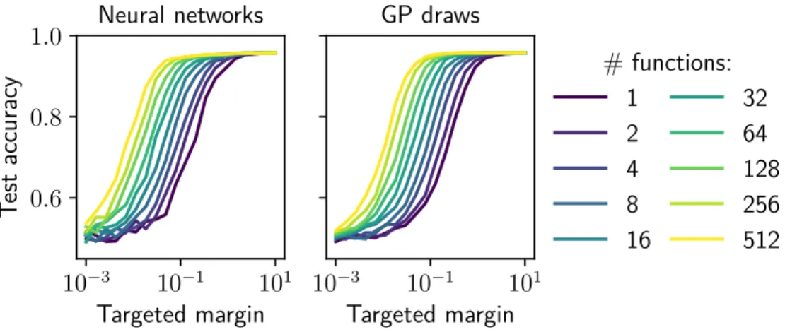
Max-margin neural networks as Bayes point machines
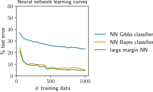
Gaussian process posterior, and taking this normalized margin to infinity, the posterior focuses on a minimal RKHS norm kernel interpolator. Qualitatively similar behavior was observed in both cases: the average of many features with a small normalized margin achieved similar accuracy as one feature with a large normalized margin. The main visible behavior is that one function of a large normalized margin appears equivalent to the average of many functions of a small normalized margin.
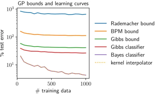
Empirical comparisons between classification strategies
The Bayes classifier and the kernel interpolator achieve inseparable performance, supporting the claim that the minimum RKHS norm kernel interpolation is a Bayes point machine. Despite the kernel interpolator performing significantly better than the Gibbs classifier in practice, the order of the Gibbs and BPM bounds is reversed.