Introduction
Introduction
In the second category, no change is made to the mass matrix of the ring polymer, that is, the equations of motion are not predetermined [13,16–. In the present study, we focus on the accuracy of both statistical and dynamic properties of the OBABO and BAOAB schemes, as well as the corresponding integrators obtained when the exact free ring polymer step is replaced by the strongly stable Cayley modification ( OBCBO). and BCOCB, respectively).
Non-preconditioned PIMD
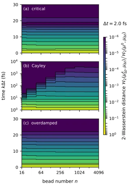
The standard method for discretization Eq. 2.8) is to use a symmetric splitting method in the form of Eq. 2.1) which consists of a combination of three types of sub-steps: i) exact free ring-polymer evolution of time stepτ,. Asn → ∞ this maximum safe time step goes to zero, so that no finite time step for the scheme in Eq. 2.1) is secure against non-ergodicity within this limit.
BCOCB avoids pathologies in the infinite-bead limit
For the Cayley modification of Eq. 2.21) still provides a sufficient condition for ergodicity, except with. The variances in the position and velocity margins of the numerical stationary distribution with the covariance matrix in Eq. 1In the special case where Λ = 0, the given condition for OBCBO corrects a sign error in Eq.
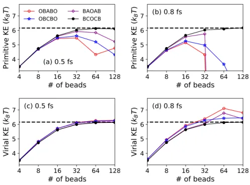
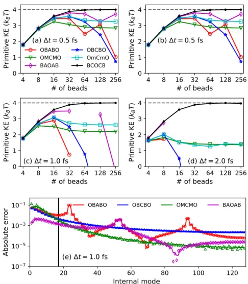
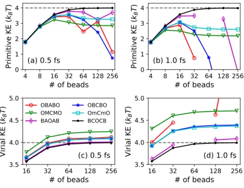
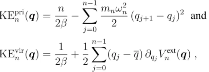
Consequences for the primitive kinetic energy expectation value
For various MD time steps∆t, the primitive kinetic energy expectation value as a function of the number of ring-polymer beads, with the exact kinetic energy indicated as a gray dashed line. Equations (2.32) and (2.33) indicate that the primitive kinetic energy estimator is a sensitive measure of the finite-time-step error in the sampled ring-polymer position distribution associated with the high-frequency modes.
Dimensionality freedom for OBCBO via force mollification
Even within the functional form of the softening in Eq. 2.35), flexibility remains regarding the choice of matrixΩ˜, which allows mode specificity in how the softening is applied. A simple choice for this matrix is Ω˜ =Ω, so that mollification is applied to all non-zero internal modes of the ring polymer.
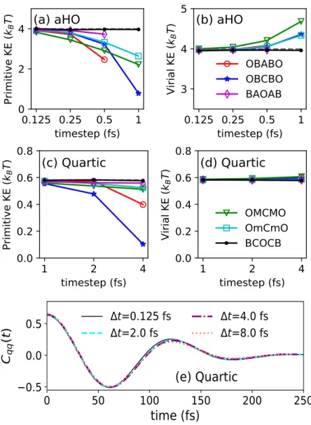
Results for anharmonic oscillator
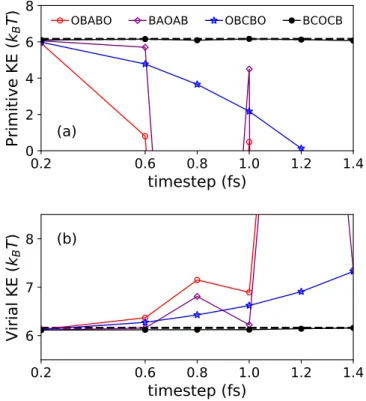
While the virial kinetic energy for all strongly stable integration schemes is well conserved, the OBABO and BAOAB schemes perform erratically on large time steps due to their provable non-ergodicities [26]. Attractively, the BCOCB scheme is consistently more accurate for the expected value of the virial kinetic energy, as it was for the expected value of the primitive kinetic energy.
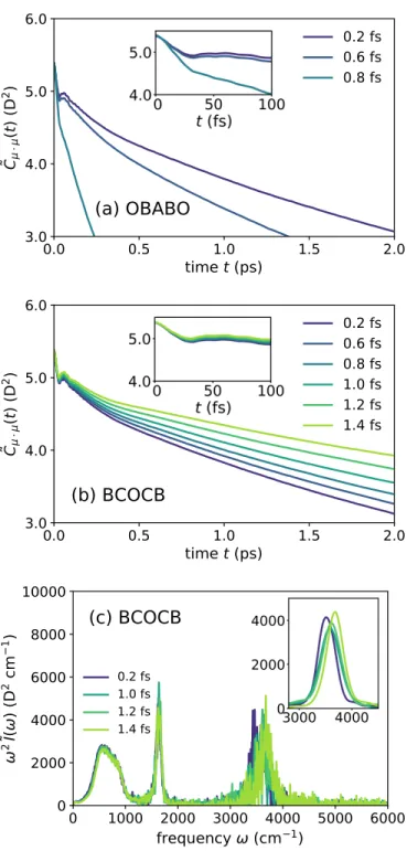
Results for liquid water
For the smallest time step of 0.5fs, which is a common choice for water path integral simulations, all integrators perform similarly. The reference kinetic energy, converged over a staging PIMD simulation at time step ∆t = 0.1 fs and 256 beads, is shown by a dashed line. The reference kinetic energy, converged over a staging PIMD simulation at time step ∆t= 0.1fs and 256 beads, is shown by a dashed line.
For the BCOCB integrator, the resulting correlation functions are much more robust with respect to time steps.
Summary
Dynamic properties of liquid water calculated using T-RPMD with (panel a) OBABO and (panels b and c) BCOCB integration schemes. Panels a and b present the Kubo-transformed dipole autocorrelation function calculated with different time steps, and panel c presents the absorption spectrum from the BCOCB correlation function at each time step. The numerical performance of the BCOCB scheme is particularly striking, providing results that are significantly better in terms of accuracy and time-step stability than any of the other integrators considered.
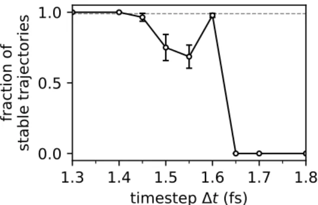
For liquid water, it is shown that BCOCB allows time steps of up to 1.4 fs, while causing minimal time step error in the calculation of both equilibrium expectation values and the dipole absorption spectrum.
Appendix A: Other splittings
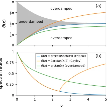
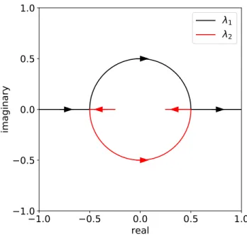
Spectral properties of the T-RPMD update for the free ring polymer for different choices of θ. If the evolution of the ring polymer is governed by the BAOAB-like update in Eq. Zhou, “Continuum limit and preconditioned Langevin sampling of the path-integral molecular dynamics,” Journal of Computational Physics.
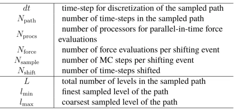
L total number of levels in the sampled path lmin the finest sampled level of the path.
Generalization and optimization of dimension-free integrators for
Introduction
The first approach introduces a preconditioned form of the equations of motion by varying the ring-polymer mass matrix. Preconditioning improves the stability of the accurate update of the free ring and polymer at the expense of consistent dynamics. In addition to the strong stability of the free update of the polymer ring, another basic requirement of a numerical integrator for T-RPMD is non-zero overlap between digits.
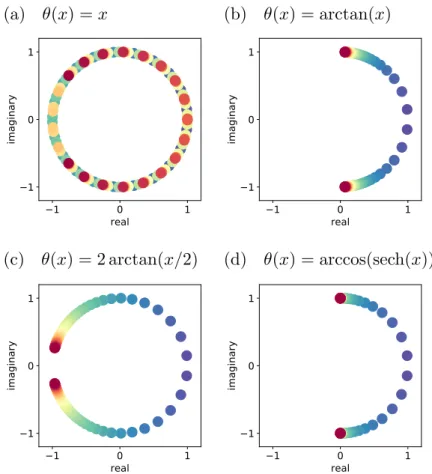
To this end, we introduce a function θ that defines the free update of the polymer ring and infer how the choice of θ affects the properties and performance of the corresponding T-RPMD integrator.
Theory
We proceed to identify sufficient conditions on θ so that the corresponding update of the free ring of the polymer satisfies property (P1). The latter choice leads to the Cayley approximation of the ring-polymer free update, as can be verified by substitution in Eq. This distribution corresponds to the jth marginal of the free-ring-polymer equilibrium distribution with density proportional toexp(−βHn0(q,v)).
This update can be interpreted as a symplectic perturbation of the free ring–polymer update in Eq. 3.7) due to the harmonic external potential [26], and preserves a modification of Hj,n that depends on the choices of θ and∆t[67].
Numerical results
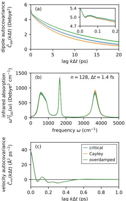
Figure 3.4 compares the accuracy and efficiency of different BAOAB-like T-RPMD schemes at equilibrium as a function of the bead number n. For a description of the numerical simulation and statistical estimation procedures used to generate the numerical data (filled circles) in Fig.3.4, the reader is referred to Sec.3.11. For these two observables, Fig. quantifies 3.4b and 3.4d the equilibrium sampling efficiency of the schemes in terms of the integrated autocorrelation time (or normalized asymptotic variance) [70–74].
Figures 3.4a-d show that the scheme specified by the Cayley angle (orange) outperforms others in terms of both accuracy and efficiency in estimating the equilibrium average of the observable quantum kinetic energy.
Summary
On the scale in which the absorption spectrum displays its key features, the spectra in Fig.3.6b show very slight qualitative differences. Collectively, these observations indicate that the accuracy of dynamic properties calculated with BAOAB-like schemes is not significantly affected by the particular θ if conditions (C1)–(C4) in Sect.3.2 are met. This result is expected due to the fact that the considered dynamic properties depend on bead-averaged (i.e. centroid mode) coordinates, the evolution of which is largely independent of the choice of θ under weak coupling between the centroid and non-centroid ring polymer modes.
To conclude, we emphasize that the implementation of BCOCB or any of the new dimensionless and highly stable schemes adds no cost, no algorithmic parameters and trivial coding overhead with respect to the standard BAOAB integrator.
Appendix A: Necessary and sufficient condition for eigenvalues of a
In this way, the chapter supports the outstanding utility of BCOCB for accurate and efficient equilibrium simulation of condensed-phase systems with T-RPMD. The eigenvalue pairs either lie on the circle with radius r = 1/2 or are both real, and in the former case the spectral radius of Mis is minimal.
Appendix B: Stability condition for harmonic external potentials
Since ϵ > 0 is arbitrary and arctan is monotonically increasing, we can conclude that the theorem holds with ∆t2Λ/m < 4 andθ(x)≤2 arctan(x/2).
Appendix C: Dimension-free quantitative contraction rate for har-
The following theorem shows that from any two initial distributions µj and νj on R, the distance between the distributions µjpkj,nandνjpkj is contractive. In the case where A(ωj,n∆t)>0, we get the required result since|A(ωj,n∆t)|<1by consequence3, and therefore,. 3.29), and then taking square roots, gives the required result.
Appendix D: Total variation bound on the equilibrium accuracy error
Taking the square roots and using the Riemann zeta function [78] to evaluate the infinite sum gives Eq.
Appendix E: Asymptotic variance of kinetic energy observables for
In the following, we denote both observers in Eq. 3.34) ask and differentiate between the two as necessary. Therefore, in the limit of infinite friction, where Mj,n,∆tis given in Appendix 3.7, the time integrated autocorrelation of KE evaluates to. Therefore, because it gives the largest stable angle, choosing θ(x) = 2 arctan(x/2), which corresponds to the Cayley angle, minimizes the upper bound in Eq.
A similar argument can be made to support the conjecture, suggested by Fig.3.4f, that the non-centroid velocity estimator for the classical kinetic energy KEclan in Eq. 3.5), exhibits a maximum integrated autocorrelation time if the Cayley angleθ(x) = 2 arctan(x/2) is used.
Appendix F: Stability interval calibration for liquid water simulations 68
Manolopoulos, "Quantum diffusion in liquid water from ring polymer molecular dynamics," Journal of Chemical Physics. Manolopoulos, "Quantum diffusion in liquid para-hydrogen from ring-polymer molecular dynamics," Journal of Chemical Physics. Manolopoulos, “How to remove spurious resonances from ring polymer molecular dynamics,” Journal of Chemical Physics.
Manolopoulos, "Chemical reaction rates of ring polymer molecular dynamics", The Journal of Chemical Physics.
Introduction
Method
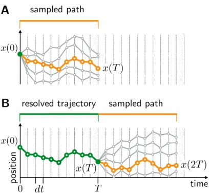
However, before addressing efficiency, Fig.4.4 illustrates that the integration scheme in Fig.4.2 is a non-equilibrium relaxation process for the segments of the sampled path. The above considerations suggest that the scheme in Fig.4.2 can lead to reduction of the wall clock time associated with MD integration, compared to standard methods. For a general implementation of the integration scheme in Fig.4.2, the expression forχ is obtained as follows.
Equation (4.8) shows that the path-based integration scheme in Fig.4.2 offers the possibility of reducing the wall clock time required for calculating MD trajectories, compared to conventional stochastic MD.
Calculation details
Random fragmentation of the pathway is performed between MC steps, so that fixed system positions at previous fragment endpoints can be sampled during subsequent steps (Fig.4.5C). Despite these choices, the sampling remains ergodic due to the random fragmentation of the path that occurs between MC steps [38,54] . The new fragmentation of the path allows for updates of system positions held in previous MC steps.
For both harmonic oscillator and Lennard-Jones applications: regeneration of the sampled path after shifting. is run with the same distribution used to generate path sampling pilot configurations.
Results
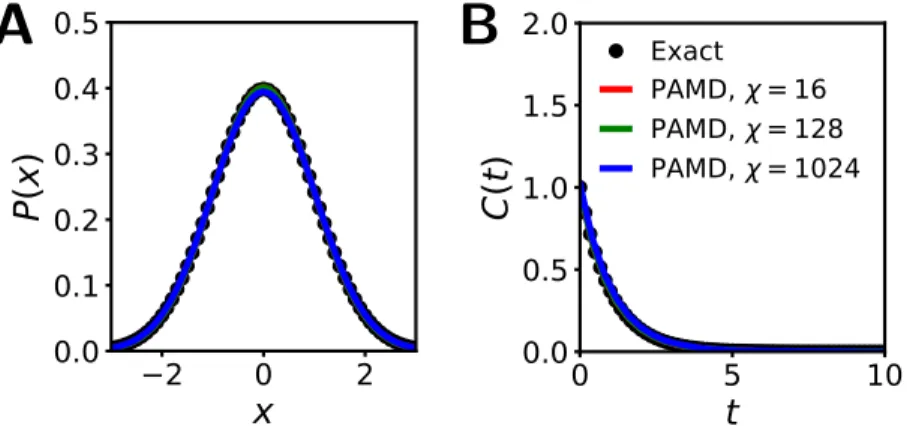
The accuracy of the PAMD trajectories is clearly preserved across all simulations, as indicated by the plotted results and the reported values of Eeq and Edyn. For all PAMD simulations reported in Tbl.4.2, a significant part of the speedup comes from the 16 times larger time step that can be used in the path-based scheme (dt = 0.4vs.dtE = 0.025). The accuracy of the integrated MD trajectories is evaluated in terms of the radial distribution functiong(r) and the self-diffusion coefficientD, using the respective error measurements.
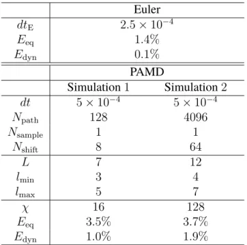
Also shown in Tbl.4.3 are two PAMD simulations leading to 16-fold (χ = 16; Simulation1) and 128-fold (χ = 128; Simulation2) reductions in the wall clock time required to generate equivalently accurate MD trajectories for Lennard-Jones fluid via the Euler algorithm using simulation parameters keeping error values below 5%.
Conclusions
Pratt, "A Statistical Method for Identifying Transition States in High-Dimensional Problems", The Journal of Chemical Physics. Andricioaei, "Directional Negative Friction: A Method for Improved Sampling of Rare Event Kinetics", The Journal of Chemical Physics. Geissler, "Conservation of Correlations Between Trajectories for Efficient Path Sampling", The Journal of Chemical Physics.
Eichhorn, "Brownian dynamics simulations with rigid-body interactions: spherical particles," The Journal of Chemical Physics.