PDF By Landen D. Ryder Thesis - Vanderbilt University

The influence of the polarization density by a material acts as a modification of the flow behavior in vacuum. Using this functional form, the refractive index remains in the complex exponential, contributing to the phase of the wave.

Lorentz Model

In the case that the nonlinear terms of the restoring force are small compared to the linear term (𝛾1𝑥 ≫ 𝛾𝑛𝑥𝑛), perturbation analysis is an attractive technique commonly applied to similar problems in quantum mechanics [18],[19]. Analogous to energy conservation, the delta function ensures that the frequency of the induced polarization density (𝜔) is the sum of the two driving frequencies (𝜔1, 𝜔2).

Free Carrier Effects

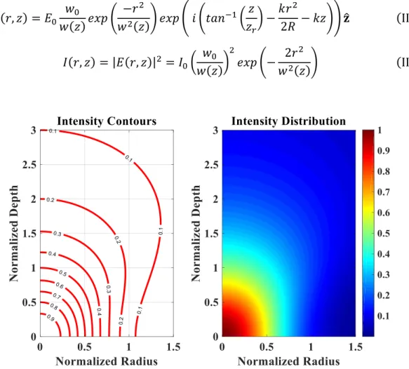
By neglecting the higher-order corrections, the total induced polarization density at this driving frequency can be rewritten. In most cases, the fundamental mode cross section of a laser can be approximated as a Gaussian radial function.

Gaussian Optics

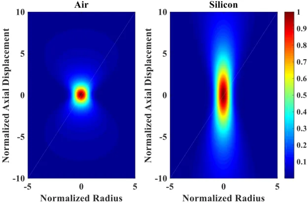
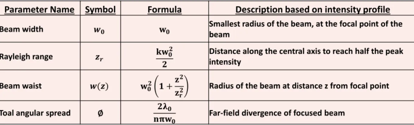
The position z = 0 corresponds to the minimal beam radius, called the beam width 𝑤0, which can be experimentally measured at the focal point of the laser beam. The Rayleigh range increases and therefore the confinement of the beam along the propagation axis decreases in higher-index materials.

Figure III.1. Spatial distribution of normalized intensity values to illustrate the spatial confinement of intensity (energy) of a Gaussian beam near the focus and its spread as it propagates away from the focus

Finite Difference Time Domain Method

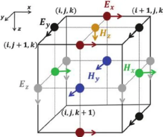
Because spatial operations, such as three-dimensional curl operations, are limited to the vertices of the grid, field components cannot be computed at the same spatial location. An illustration of the decomposition of spatial field information into field components computed at discrete locations in a spatial unit cell known as a Yee Cell. An example of the field component update equations can be seen below in Eq.

Figure IV.1. An illustration of the decomposition of spatial field information into field components that are calculated at separate locations in a spatial unit cell known as a Yee Cell

Wave modulation and generation rates

Free carrier refraction is expressed as a function of the free carrier density in the material. Considering absorption processes from single/two photon absorption and free carrier absorption, the total absorption can be expressed as the sum of the contributions of the processes. Considering refraction processes of single/two photon absorption and free carrier absorption, the total phase accumulation can be expressed as the sum of the contributions of the processes.

FDTD Implementation

8ℏ𝜔 |𝐸|4 (IV. 23) Using the free carrier concentration expression, the polarization density for free carrier refraction and free carrier absorption can be expressed as a function of the free carrier density from Eqs. The discretization of the time derivative associated with the generation of free carriers enables the creation of an update equation for the concentration of free carriers. After expanding the individual polarization densities, the discretized displacement field can be constructed to solve the electric field.

Figure V.I. Pictographic representation of the PL-SEE measurement system at Vanderbilt University [30]

Simulation Mesh

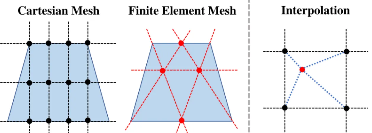
However, there are cases where the lumeric mesh needs to be adjusted in the sub-areas of the simulation. A "Mesh Override" region defines a spatial extent in which the spatial step size in each Cartesian direction can be specified, independent of the meshing routine invoked for the simulation. Although there are clear advantages to using mesh overrides, care must be taken as continuity requirements for the Cartesian mesh can result in mesh refinement in some subregions, forcing mesh refinement to be adopted in neighboring regions.

Boundary Conditions

The discrete refractive index spectrum of a material can be measured experimentally (for example, by ellipsometry [47]), taken from the literature [48], or generated from an analytical model (such as optical conductivity), which can be used to generate a numerical model that is used for material in simulations. For each material, the dielectric function defined in the frequency spectrum of the simulation range can be plotted to check the quality of the analytical model. Each material model instance can be created with a base material such as silicon and a parameterized model such as the Kerr coefficient.

Sources

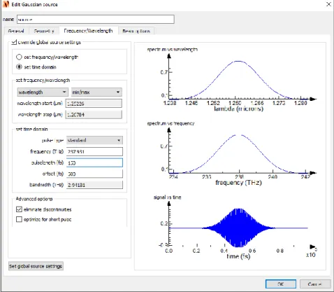
Temporal behavior of the pulse can be specified in either the temporal or the frequency domain, with corresponding parameters calculated for the unspecified domain. Offset: Time between the start of the simulation and the maximum amplitude of the pulse [fs]. GUI used to parameterize the temporal/frequency content of the laser pulse injected into the simulation.

Figure V.III. GUI used to parametrize the temporal/frequency content of the laser pulse injected into the simulation

Monitors

The temporal behavior of the field components can be stored by including time monitors to capture the response of the device to a specific, user-defined excitation. Field component postprocessing produces the spectral density of the fields at each spatial node that can be stored by frequency monitors in a manner similar to a time monitor. As discussed earlier, the spectral density of the pulse and corresponding fields can be expressed as 𝑠̃(𝜔) and 𝐸⃗⃗𝑠𝑖𝑚(𝜔), respectively.

Post Simulation Processing

It is essential to understand the implications of reducing 3-D simulations to 2-D simulations in order to verify the validity of the reduction as well as to interpret the simulation results appropriately. From the Courant stability condition, the maximum time step is calculated internally as a function of the materials and spatial size of the meshes and cannot be modified by the user. By default, the maximum temporal step is used to minimize the wall time of the simulation, but in some situations it is necessary to decrease the temporal step to increase the robustness of the simulation.

Tool Suite Overview

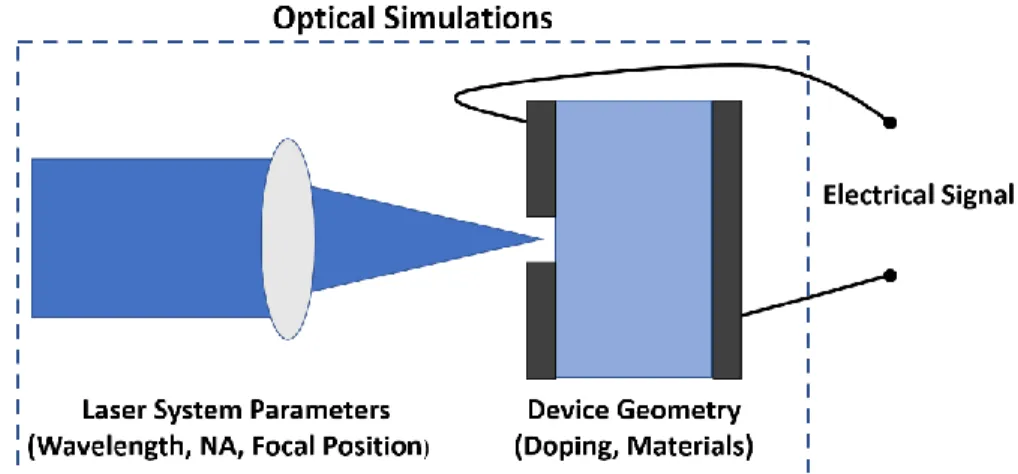
From the perspective of simulating PL-SEE testing, optical simulations capture the optical pulse passing through a device and depositing a spatial distribution of charge within a device. Therefore, to fully model a PL-SEE from laser pulse to measurement, the simulated spatial distribution of the charge from the pulse must be used as an initial condition in a charge transport code. The spatial distribution of charge in a device, whether mobile or immobile, induces an electrostatic potential distribution that can be described by the Poisson equation [49].

Generation Models

Computational techniques for computing optically generated carrier distributions, including FDTD and beam propagation solvers that can be called before or during a device simulation, are available from the. Temporary envelopes that are nonzero only at a subinterval of the simulation time can be used to inject a finite amount of charge distributed over the subinterval, such as an appropriately defined Gaussian or square pulse. From this functional form, the scale factor can be calculated by integrating 𝐹(𝑡) to 1.

TDR Files

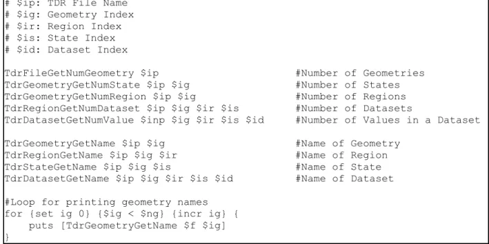
TdrFileGetNumGeometry $ip #Number of geometries TdrGeometryGetNumState $ip $ig #Number of states TdrGeometryGetNumRegion $ip $ig #Number of regions TdrRegionGetNumDataset $ip $ig $ir $is #Number of datasets. TdrDatasetGetNumValue $inp $ig $ir $is $id #Number of values in the dataset TdrGeometryGetName $ip $ig #Geometry name. TdrRegionGetName $ip $ig $ir #Region Name TdrStateGetName $ip $ig $is #State Name TdrDatasetGetName $ip $ig $ir $is $id #Dataset Name.

Command File

TdrDataGetCoordinate $ip $ig $ir $is $id $iv 0 #X Coordinate of Node TdrDataGetCoordinate $ip $ig $ir $is $id $iv 1 #Y Coordinate of Node TdrDataGetCoordinate $ip $ig $ir $is $id $ iv 2 #Z Coordinate of Node TdrDataGetValue $ip $ig $ir $is $id $iv #Quantity value at Node. The "File" section relates to the file management associated with a device simulation, with specific keywords for defining input/output files for specific applications. Many physical models are defined with default material-dependent parameters that can be overridden by including parameter files, containing user-defined model parameters, in the "File" section using the "Parameter" keyword.

Integration with Lumerical

After completing the simulation tools, comparison with analytical models and experimental results is essential to establish the validity of the tools. Simple analytical models can be used to verify the accuracy of the free carrier optical models and the effect of doping profiles on the optical simulations. The benefit of the first-principles approach to the optical simulations on the experimental results is also discussed in this chapter.

Figure VI.9. For the same spatial distribution, two distinct meshes (black and red) can used to discretize the spatial extent into sets of nodes

Incorporated Free Carriers

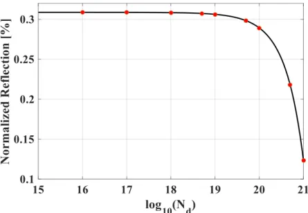
Using the free carrier refractive parameters defined for silicon, the reflection coefficient of the doped material can be simulated as a function of the doping concentration. Neglecting free carrier generation processes implies that the free carrier density of the material is determined by the doping concentration 𝑁𝑑𝑜𝑝𝑖𝑛𝑔 of the material. A strong agreement between the simulations and the analytical models confirms the correct implementation of the free carrier absorption models within FDTD Solutions.

Figure VII.1. Reflection coefficient from free carrier refraction as a function of doping level

Pulsed Laser Testing on a Silicon Diode

A free carrier absorption cross section of 10−22 𝑚2 was used to simulate normalized intensity-depth profiles as a function of doping density, plotted in Figs.

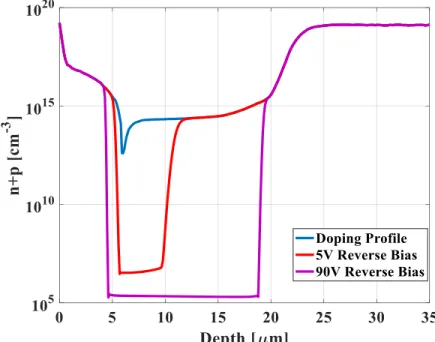
Doping Profile

Distribution of free carriers in a silicon diode (Figure VII.3) in equilibrium for reverse bias conditions: dopant profile (without bias), 5 V and 90 V. From the distribution of the free carrier density, the corresponding distribution of absorption coefficients and refractive index modulation can be calculated with using the FCA model in silicon (equation IV.10). Since free carrier densities associated with doping levels in the active region of a typical device result in minimal free carrier absorption, local reductions in carrier densities near material junctions only further reduce free carrier absorption.

the same process as Eqn. VII.4, Fig. VII.4 contains the total free carrier density as a function of depth in the silicon diode (Fig

Optical Simulations

TCAD Simulations

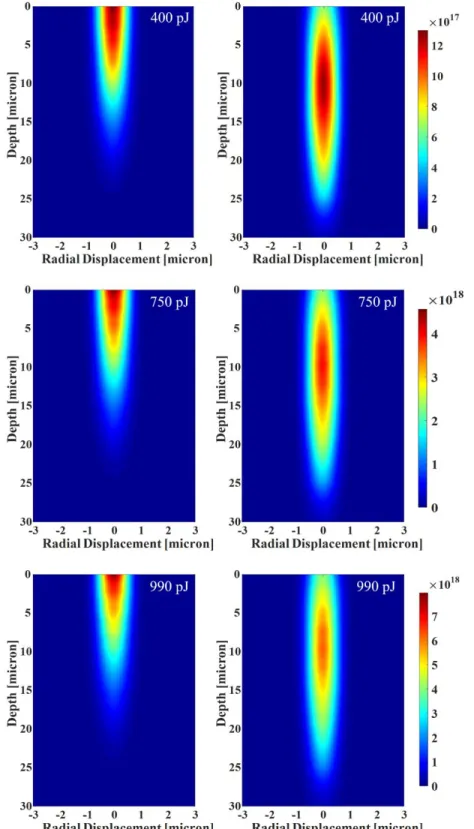
Silicon diode depth profiles for three pulse energies for two reverse bias conditions: 5 V (left) and 90 V (right). By using mixed-mode TCAD simulations to capture circuit components related to the measurement system, such as bias connections, the entire pulsed laser measurement technique, from the laser pulse to the electrical response of the device, can be emulated in the simulation environment. This approach allows comparison of the simulated current transition with the experimental current transitions, with the example shown in Fig.

Figure VII.6. Cross sectional cut of optically generated carrier distributions for three different pulse energies: 400 pJ, 750 pJ, and 990 pJ

Advantages of FDTD

This simulation approach breaks down PL-SEE testing into optical simulations to account for charge deposition from a laser pulse and charge transport simulations of the deposited charge. The functionality of the solver related to the simulation of charge deposition by a laser pulse is highlighted (Chap. V). Integrating optical simulations with a charge transport solver creates a simulation infrastructure that models pulse-to-electric signal PL-SEE testing.