ON THE IMMERSED FRICTION STIR WELDING OF AA6061-T6: A METALLURGIC AND MECHANICAL COMPARISON TO FRICTION STIR
WELDING
By
Thomas Bloodworth
Thesis
Submitted to the Faculty of the Graduate School of Vanderbilt University
in partial fulfillment of the requirements for the degree of
MASTER OF SCIENCE in
Mechanical Engineering May, 2009 Nashville, Tennessee
Approved:
Professor Alvin M. Strauss Professor George E. Cook
Dr. David R. DeLapp
For my parents Charles and Janet Bloodworth and my fiancée Kristie Adkins
ACKNOWLEDGEMENTS
I would first like to thank God on whose constant intersession and peace I rely on for help. I would also like to thank the people and organizations whose efforts and contributions made this work a success. My graduate committee Drs. Al Strauss, George Cook, and Dave DeLapp; my fellow researchers in the welding lab; Paul Fleming for designing the automation and interfacing software which makes running the welding machine much safer and simpler, David Lammlein, Tracie Prater, Paul Sinclair for his help with 3-D CAD; Bob and John from the Physics machine shop; Drs. Art Nunes and Alan Chow from Marshall Space Flight Center for private communications and NASA GSRP funding for this project; Tennessee Space Grant Consortium for additional stipend and tuition support; all my undergraduate professors especially my physics professors and advisors Drs. Alex King and Jaime Taylor; my family, friends, and loved ones for there patience, love, and support they have given for my efforts. No one has been as motivating and inspirational as my parents, Charles and Janet, my brothers, Charles Jr., Aaron, and Eric, and my fiancée Kristie.
TABLE OF CONTENTS
Page
DEDICATION... ii
ACKNOWLEDGEMENTS... iii
LIST OF TABLES ... vi
LIST OF FIGURES ... vii
LIST OF ABBREVIATIONS... ix
Chapter I. INTRODUCTION ...1
Thesis Objective...1
Overview of the FSW Process ...2
Applications and Advantages ...2
II. LITERATURE REVIEW...4
FSW Terminology ...4
Process Parameters...5
Weld Zone Regions...5
Weld imperfections, flaws, and defects ...7
Friction Stir Welding Tool Contributions...9
Weld Pitch...13
Porosity ...14
Submerged Friction Stir Processing...15
Underwater Friction Stir and Rotary Friction Welding ...20
III. EXPERIMENTAL PROCEDURE ...27
Thermocouple Implantation...31
Experimental setup for threaded cylinder ...33
Tank Construction...35
IV. EXPERIMENTAL RESULTS FOR THE THREADED PROBE TOOL...36
V. EXPERIMENTAL RESULTS FOR THE TRIVEX PROBE TOOL...40
Axial Force...40
Torque ...43
Power ...44
Heat Input as a Function of Welding Process ...46
Materials Testing ...47
VI. FINITE ELEMENT MODEL OF STEADY STATE WELDING TEMPERATURE BASED ON FORCE DATA...51
Background ...52
Description of the Model ...54
Results and Comparisons...57
Discussion and Conclusions ...60
Appendix A. Raw Force and Moment Plots for Control Welds...63
B. Raw Force and Moment Plots for Underwater Welds ...75
C. Raw Data used in Finite element analysis...86
REFERENCES ...89
LIST OF TABLES
Table Page
1. Advantages of friction stir welding...10
2. Composition and properties of AA6061-T6 ...16
3. Data gathered by Hofmann and Vecchio ...19
4. Composition of 0 – 1 oil hardened tool steel ...34
5. Force and data from the threaded probe experiment ...39
6. Weld matrix for Trivex tool experiment...40
7. Elemental composition of H13 tool steel...54
LIST OF FIGURES
Figure Page
1. Schematic of the friction stir welding process ...2
2. Plane View of FSW zones ...6
3. Typical void defect in FSW ...7
4. Flash occurring on the retreating side of a FSW...8
5. Joint line remnant at the root of the joint line...9
6. Joint line remnant in the weld nugget ...9
7. Tool geometries from Elangovan and Balasubramanian ...11
8. Different flow regimes in FSW (Schneider et al., 2006) ...12
9. Experimental setup from Hofmann and Vecchio for SFSP ...17
10. Thermocouple data from multiple passes of SFSP in AA6061 ...18
11. Grain structure in FSP and SFSP ...20
12. U-bend test samples from Clark ...21
13. Crack growth in UWFSW of steel ...22
14. Crack growth in FSW of steel...23
15. Minimum hardness vs. Maximum T in FW AA6061 ...24
16. Joint efficiency vs. welding time ...25
17. Joint efficiency vs. lowest hardness...25
18. FSW machine at VUWAL ...27
19. Tool dimensions for both experiments ...28
20. Trivex parameters vs. area ratio...29
21. Triflute, Triflute – MX, and Trivex tools ...30
22. Thermocouple hole dimensions ...31
23. Water tank ...35
24. Tensile test schematic ...37
25. Tensile specimens from the threaded probe matrix ...38
26. Axial force vs. travel speed for 1000-2000 rpm ... 41-42 27. Moment vs. travel speed for 1500 and 2000 rpm ... 43-44 28. Power vs. travel speed at 2000 rpm ...45
29. Heat Input vs. IPM for IFSW...46
30. Heat Input vs. RPM for IFSW ...47
31. Hardness vs. nugget location ...48
32. Root flaw for FSW and IFSW ...49
33. UTS vs. rotation speed for IFSW...50
34. Temperature dependent yield strength of AA6061...52
35. Tool used in steady state model and experiment ...54
36. Isometric view of finite element mesh...55
37. Boundary conditions for the FEA ...56
38. Load values for FEA...56
39. Temperature isotherms for 1500 and 3500 rpm...58
40. Maximum temperature vs. time for 1500 rpm at 30 ipm...59
41. Maximum temperature vs. time for 3500 rpm at 30 ipm...59
42. Temperature as a function of distance from pin bottom ...62
LIST OF ABBREVIATIONS
Symbol or Abbreviation
IFSW / SFSW Immersed (Submerged) Friction Stir Welding FSW Friction Stir Welding
FSP Friction Stir Processing
SFSP Submerged Friction Stir Processing UTS Ultimate Tensile Strength
IPM Inches per Minute
RPM Revolutions per Minute
Fx Force along traversing direction
Fy Perpendicular to Fx and Fz
Fz Force along rotational axis
Mz Moment or torque about the rotational axis w rotational velocity (spindle speed)
r material density
k thermal conductivity
T temperature
Cp specific heat at constant pressure
FEA Finite Element Analysis
FEM Finite Element Method
VUWAL Vanderbilt University Welding Automation Lab
CHAPTER I
INTRODUCTION
Thesis Objective
The objective of this research was to quantify the material properties as well as the forces unique to immersed friction stir welding (IFSW) as compared to conventional friction stir welding (FSW) performed in air of AA6061. These results were compared by using ultimate tensile strength (UTS) and weld root properties such as joint line remnant length at the interface between the welded aluminum alloy which allows crack initiation.
Metallurgic cross sections of the AA6061 welds were prepared and the weld nugget hardness between the two welding techniques was compared as well.
In order for the IFSW technique to be viable as a means to not only improve nugget hardness and reduce the grain size in the recrystallized zone or nugget, but to improve weld strength. Experiments such as this one and others quantifying the forces and process parameters must be performed. The immersed friction stir welding process should be thought of as a beneficial in-situ heat treatment. A steady state model of
temperature distribution has been put forward and is shown to accurately predict trends in heat input using heat generation equations from Schmidt et al. [Schmidt et al., 2004]
[Schmidt and Hattel, 2005]. Temperature distribution was measured and correlated to data by use of Micron Thermal Imaging camera.
Overview of the FSW Process
Friction stir welding was invented and patented by a research team led by Wayne M. Thomas [Thomas et al., 1991] [Thomas et al., 1995] of the Welding Institute in England. FSW is defined by Threadgill of TWI as “…a method for joining two or more work pieces where a tool, moving in a cyclic manner relative to the work pieces, enters the joint region, locally plasticizes it and moves along the interface thus causing a solid state joint between the work pieces” [Threadgill, 2007]. A schematic of the friction stir welding process is shown below in figure 1. It can be observed that that, due to the rotation of the tool, friction stir welding is an asymmetric process with respect to the joint line.
Figure 1: Schematic of the Friction Stir Welding Process [Mishra and Ma, 2005]
Applications and Advantages
Friction Stir Welding is primarily used to bond aluminum alloys and light weight non-ferrous alloys such as magnesium. FSW has an advantage over conventional arc welding by bonding the joint in the solid state. Arc welding processes melt the weld pool
producing large grained brittle joints as the nugget recrystallizes from liquid to solid.
Additional post processing techniques such as heat treatment are sometimes required to anneal the metal to reduce the high residual stresses and distortions produced by a multiphase joining process.
NASA uses FSW on Al-Li 2195 for the production of external fuel tanks for the shuttle as well as the Aries launch vehicle for space exploration [Prater, 2008]. Other industries using friction stir welding for joining include the aerospace, railway, automotive, shipbuilding/marine, and construction industries.
CHAPTER II
LITERATURE REVIEW
Friction Stir Welding Terminology
TWI has set standards for referring to the various processes and parameters used in friction stir welding [Threadgill, 2007].
The tool is defined as the rotating piece designed to generate heat, plastically deforming the weld material in order to form the bond. This definition is generalized as various tools exist with a floating, fixed, or stationary shoulder geometry thus generating no heat for the purposes of welding. The probe is the part of the tool which is plunged below the surface of the work piece being welded. It may or may not be “pin-shaped” and may or may not exist depending on the application. The shoulder of the tool rests on the surface of the material being welded and may be plunged slightly into it. The shoulder is always of a smaller diameter than the probe.
The leading and trailing edge terminology used as an analog to airfoils, Threadgill points out, is misleading due to the fact that most tools are cylindrical and therefore due not have edges. The terms leading face and trailing face will be used to distinguish between the front and rear limb of the tool as the front is described as the direction of travel. In the event that the tool is tilted away from the direction of travel and the shoulder is plunged into the material, the portion of the shoulder under the material is called the heel and the angle of the tool with respect to the vertical is known as the tilt angle or travel angle. The amount the tool shoulder is plunged into the work piece is
known as the heel plunge depth. Tool features such as scrolls, flats, thread, etc. have been defined, says Threadgill, adequately though alternative use and thus continued usage of these terms is permissible.
Process Parameters
Processing parameters for friction stir welding including rates of travel, rotation, and forces will be explained here. Threadgill uses welding speed as an alternative to traversing rate or traversing speed. Similarly, the rotational velocity of the tool is known as the tool rotation speed. Its direction of rotation, clockwise or counter-clockwise, is described when observing the tool from above.
The force parallel to the rotational axis (or Z axis) is known as the down force or axial force. The force parallel to the travel axis is known as the traversing force and lies in the X direction. The force in the same plane and orthogonal to the traversing force is known as the side or lateral force.
Weld Zone Regions
The advancing side and retreating side are important to point out in the cross section, or plan view, of a weld. This is due to the fact that friction stir welding is inherently an asymmetric process because of the rotational velocity and features of the tool. The advancing side is the side of the weld which the rotational velocity component and traversing velocity component are constructive or additive. The retreating side is the side of the weld which the rotational velocity component and traversing velocity
component are destructive or subtractive.
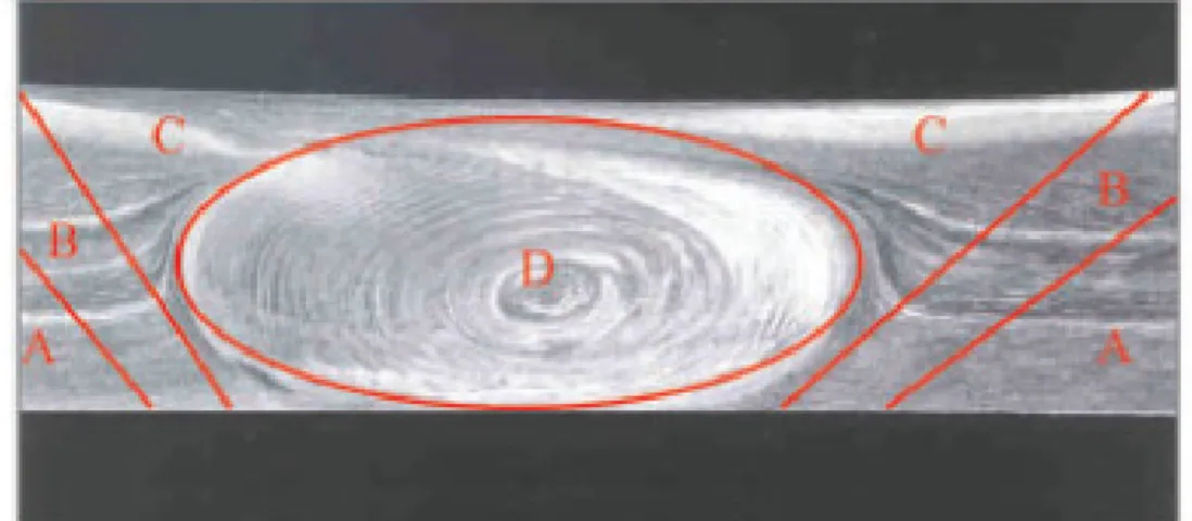
Weld features and zones will be identified using the plan view illustrated in figure 2. The four main zones are listed below and are labeled A, B, C, and D. These are the primary zones for describing the amount or lack of thermoplastic heating and mixing of the weld joint. The descriptions of the zones A-D are defined below.
Figure 2: Plane View of FSW zones
The zone labeled ‘A’ in the above figure is known as the parent material. This is the region farthest from the joint center line and has not been affected by heat or
deformation. Area ‘B’ is affected only by heat and no plastic deformation is visible. This zone is known as the HAZ or heat affected zone which parallels fusion welding
terminology. Zone ‘C’ is affected by both heating and thermoplastic deformation. It is referred to as the TMAZ or thermo-mechanically affected zone. It generally corresponds to the region of the weld under the shoulder on the top to the pin radius on the bottom of the weld. The recrystallized structure is found in the fourth major zone ‘D’ called the nugget. As a minimum the nugget is the region of heaviest mixing and therefore is found within a pin radius at least from the `joint line of the weld. The TMAZ and nugget are
both subjected to mixing and therefore can be difficult to separate in plane view sections.
This is especially true in soft metals such as aluminum alloys which are used in the work.
Weld Imperfections, Flaws, and Defects
Various imperfections were observed in the FSW and IFSW of aluminum alloys used in this study. Voids are caused by lack of material flow and can appear at the weld surface or below it and are detectable by microscopy. Porosity can be found in immersed friction stir welds as the gas bubbles create voids in the nugget and TMAZ. This is analogous the fusion welding done in inert gases in which the weld pool dissolves gas into it inducing porosity during resolidification. Generally speaking in FSW there is no porosity at low rotation and travel speeds due to the solid state process. An example of the void defect from Threadgill can be found below in figure 3.
Figure 3: Typical void defect in FSW
The flash defect is found on the surface of the weld most commonly on the retreating side. It is found on the edge of the shoulder footprint and is caused by excess heating of the weld surface leading to inadequate forging of weld metal at the heel of the shoulder. Flash was found to be easily contained by the IFSW process due to its ability to
quench aluminum quickly. An example of flash is found in figure 4. The retreating side of the weld is on top as is the flash defect.
Figure 4: Flash occurring on the retreating side of a friction stir weld
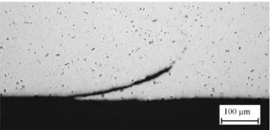
Defects can occur when the joint line is not properly mixed resulting in the joint line remnant. The remnant is a traceable joint line that has been deformed, but not mixed leaving a section of unbonded material observable on weld plan views. It is very common in single pass FSW since the probe does not mechanically mix the root of the joint line.
This can be alleviated by proper tool position, force control, and geometry of the
experimental setup. Joint line remnants can be found within the weld nugget as well and are generally not as weak as root joint line remnants. Examples of both types of joint line remnants can be found in figures 5 and 6.
Figure 5: Joint line remnant at the root of the joint line
Figure 6: Joint line remnant found in the weld nugget
Friction Stir Welding Tool Contributions
Tools used for FSW usually are composed of two main parts: a cylindrical shoulder and probe of an always lesser radius. Experiments determining heat generation and forces during FSW were run to determine various contributions of the tool features [Dubourg and Dacheux, 2006]. Frictional deformation by the tool raises the temperature
of the aluminum to a state which is plastic-like yet still in the solidus regime. Advantages of the friction stir welding process due to advances in tool design and process parameter optimization were also observed [Mishra and Ma, 2005]. Advantages over arc welding include the joining of aluminum alloys such as the 2XXX and 7XXX series alloys. These aluminum alloys are considered “unweldable” by fusion welding. The metallurgic, environmental, and energy benefits of FSW are listed in Table 1 [Mishra and Ma, 2005]
[Fleming, 2009].
Table 1: Advantages of friction stir welding
The heat input in FSW observed by Mishra and Ma, Fleming, and Dubourg and Dacheux was comparable in magnitude to fusion or arc welding techniques. However, in FSW the heat input is distributed over a larger area of the joint. This produces a joint with low residual stress and distortion due to the low temperature gradients and welding temperatures. Fusion welding has high thermal gradients and welding temperatures since it melts the weld joint to make the bond.
Pin contributions have been analyzed by a number of researchers and the
optimization of the tool is found to have great variance in the tool pin force contributions
and weld quality during welding [Elangovan and Balasubramanian, 2008]. Estimations on the contribution to axial forces during welding have ranged from 2-51% depending on the literature [Dubourg and Dacheux, 2006]. Most authors observe or model a pin
influence of less than 5% on heat input and power [Schmidt et al., 2004]. The optimal probe shape as observed by Elangovan and Balasubramanian is the square probe. This was found to be the most optimal over a wide parameter matrix using various tools including smooth probe, triangular, square, threaded among others. Figure 7 shows the various tools used in that study including the geometries used to determine optimal probe shape.
Figure 7: Tool geometries from Elangovan and Balasubramanian
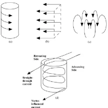
Flow around the tool is described as the superposition of 3 separate flow regimes [Schneider et al., 2006]. The illustration of the various regimes as generated by a rotating cylinder can be shown in figure 8.
Figure 8: Different flow regimes in FSW (Schneider et al., 2006)
It can be shown that the three incompressible flow fields exist forming a rotating plug of material during the welding of Al-Li 2195 observed by Schneider et al. Lead tracer material was placed in the joint line. The path of the tracer particles was analyzed by x-raying the specimen after welding. This flow is found to be driven by the threads or other features on the pin. The vertical flow contribution is easily observed by welding using the same threaded tool in both directions during successive runs and observing material flow up the pin and appears as flash at the surface. This also serves to generate a void visible by simple inspection through the entire weld nugget in the material as
observed by Paul Sinclair and others at Vanderbilt University Welding Automation Laboratory.
Weld Pitch
Weld pitch, WP, is often used to characterize a welding envelope and determine defect trends due to hot or cold welding [Crawford, 2005]. It can be misleading however to solely use weld pitch to classify a matrix. WP is simply the ratio of the rotational speed to the travel speed and has units of rev/inch (rev/mm). The first experimental matrix given later uses a range of weld pitch from 1000/14 = 71.4 rev/inch to 2000/5 = 400 rev/inch (rpi). The weld pitch can give a general trend for the expected quality of the friction stir weld. A low weld pitch indicates that the travel speed is relatively high in comparison to the rotational speed. This leads to a weld with a low heat input and poor mixing. Such welds can be expected to form worm holes at the base of the pin where temperatures are lowest and mixing is poor. The high end of the weld pitch spectrum indicates that the travel speed is relatively low compared to the rotational speed. This can lead to discontinuities discussed by W. Arbegast related to the overheating of the weld zone such as excess flash, expulsion, or surface galling [Arbegast et al., 2006] [Arbegast, 2008].
An optimum weld pitch is not universal. It is dependent on many factors including the welded alloy, welding tool, and other parameters. Variation in heat dissipation due only to a change in welding machine can alter the optimum pitch parameters. Also, a weld pitch may not be deterministic of weld quality in its matrix. This is to say that similar weld pitches with differing parameters may not lead to optimal welds. For example, a weld at 2000 rpm and 10 inches per minute (ipm) may have produced a good weld, however, a weld at 3000 rpm and 15 inches per minute produced a worm hole even though the weld pitch for both are 200 rev/inch. It can not be stressed enough that the
weld pitch parameter is for general envelope trends and should not be used to predict specific weld characteristics.
Porosity
Experiments were conducted to determine the effect of water depth on the
porosity of Ferro-alloys (iron based alloys) welded by traditional arc processes [Suga and Hasui, 1986] [Rowe et al., 2008]. Porosity was found to be highly dependent on the water depth. This is commonly attributed to hydrogen gas as well as iron oxidation at high pressure. Water pressure increases at a rate of 1 atmosphere for every 10m (33ft). In arc welding processes porosity is mitigated by the introduction of coatings which lower oxidation such as calcium carbonate or titanium which is a strong deoxidant. Porosity is seen to increase dramatically as a function of depth for arc welding. Similar studies must be investigated to define porosity trends in friction stir welding. Porosity in Ferro-alloys was previously observed to exceed 5% in conventional arc wet welds performed at greater than 15ft of water [Suga and Hasui, 1986]. AWS standards for wet welds (D3.6 Class B) specify a maximum allowable porosity as seen by metallographic cross section is 5%. Although no such standard exists yet for friction stir welding one can infer from the advantages of FSW that low porosity can be expected [Mishra and Ma, 2005].
Porosity is assumed to be the product of the oxidation of the fresh weld material as it is drawn to the surface by the mixing process. The pure aluminum quickly bonds to oxygen drawn from water molecules and hydrogen gas left over from the dissociation of the water creates porosity in the aluminum oxide. Due to the solid state nature of FSW it
is expected that the porosity dependence on depth would be mitigated although future research is needed in this area to quantify characteristics and process standards. Pressure at a depth of water would allow high porosity to develop more prevalently when the weld is in liquid phase. This is related to the intermolecular forces between the weld alloy molecules themselves. A higher temperature seen during arc welding leads to weaker bonds between alloy molecules which makes them more susceptible to oxidation than the lower temperature solid state process.
Submerged Friction Stir Processing
Two separate studies by Hofmann and Vecchio show that ultra-fine grains can be produced by processing the aluminum under a high quench rate fluid such as water [Hofmann and Vecchio, 2005]. The study follows the investigation by Mahoney and Lynch at DARPA which showed that friction stir processing can create much stronger bulk materials than the parent. The strength of cast nickel-aluminum-bronze was doubled by this technique. In friction stir processing (FSP) the procedure is very similar to friction stir welding with the only difference in that no material is welded, it is only thermo- plastically heated and stirred, and however, no joint is produced in FSP.
In submerged friction stir processing the entire bulk sample is friction stir processed underwater [Hofmann and Vecchio, 2005]. The grain structure in the weld zone, or nugget, was found to be finer in studies done on rotary friction welded pipe as well [Sakurada et al., 2002]. The study rotary friction welded AA6061 rods underwater proving that frictional heating was enough to join non-ferrous alloys in a high quench rate environment. When the aluminum cooled in the submerged environment, the nugget had
less time to recrystallize large grains as it was being quenched by the water. The Sakurada et al. study was able to produce welds with a stronger parent to weld strength ratio. The conventionally friction welded metal failed at 82% of the parent strength while the submerged welds failed at 86%, an increase of 4% when compared to the unwelded, or parent, ultimate tensile strength (UTS).
Using these studies Hofmann and Vecchio observed the ultra-fine grains in SFSP of AA6061. The properties of aluminum alloy, AA6061, will be important to the rest of this study and future chapters so its properties are listed in table 2.
Table 2: Composition and properties of AA6061-T6
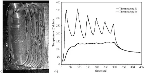
Their study was performed on a modified mechanical mill capable of spindle speeds from 60-3300 rpm. The traverse and lateral motors traveled from 0-14.8 mm/s (0- 35 inches per minute, ipm). A diagram describing the processing apparatus is shown below in figure 9.
Figure 9: Experimental setup from Hofmann and Vecchio for SFSP
The study also imbedded thermocouples to measure the temperature at the weld as well as the temperature rise of the water to determine weld heat input as a measure of enthalpy from the high quench rate process. They used 3.2 mm (1/8 inch) thick samples of AA6061 for processing. The initial grain size for the samples was found to be ~50 microns. Two tools were used and varied in shoulder size from 12.7 to 19.1 mm (1/2 to 3/4 in). The probe diameter length were kept constant at 3.18 mm and 2.79 mm (1/8 and .11 in) respectively. The process used by the study was to plunge the tool into the sample in air and process the sample underwater. This was done in order to keep the heat input into the weld as low as possible. Another processing technique was to eliminate the plunge altogether. This was accomplished by pre-drilling a recess into the parent material at the surface to accommodate the pin so that no heat was built up into the weld prior to traversing the metal.
Temperature profiles indicated by the embedded thermocouples showed that the heat input into the processed zone is similar to FSP done in air. The study hypothesizes
that this is due to the local vaporization of the water around the tool. This leaves the weld dry for a brief time until the tool progresses down the joint line and the joint is quenched by water. Temperature distribution was shown to be much more localized due to the quench rate of the underwater process. Temperature readings from successive passages of the SFSP tool show the steep gradients near the tool shoulder. These can be seen in figure 10.
Figure 10: Thermocouple data from multiple passes of SFSP in AA6061
Temperature rise was also used to determine various characteristics such as change in water temperature, temperature input, and total heat input. The heat input equation used in the study was simply an enthalpy rise of the water assuming constant volume and temperature rise. Total heat input is equal to the mass, m, of the water times the specific heat capacity, Cp, times the temperature rise, ∆T.
T mC H = p∆
∆ (1)
Table 3 tabulates the weld parameters and heat input information gathered by Hofmann and Vecchio from their initial study on SFSP of AA6061.
Table 3: Data gathered by Hofmann and Vecchio
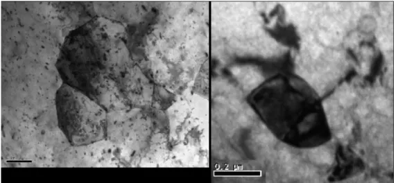
It is important to note that work did not produce any welded joints in aluminum and only reported on the grain size reduction. This was due to the fact that their study was only to improve bulk sample grain refinement in friction stir processed aluminum, not welded. Further study in the later chapters will discuss the increased nugget zone hardness and its relationship with grain size reduction. Hofmann and Vecchio’s initial study observed that the quenching of the water during processing reduced grain size in the nugget by an order of magnitude, from microns to nanometer scale. These ultra fine grains observed were on the order of 200 nm while the parent metal grain sizes were on average 50 microns. Further, more traditional FSP done in air found the grain size reduced to 5 microns or less. The order of magnitude reduction is with respect to the
grain size reduction between FSP and SFSP. The TEM micrographs of the “in air”
processed nuggets and the underwater processed nuggets can be observed below in figure 11. Future work involved using a super cooled fluid to theoretically reduce grain size to less than 100 nm.
Figure 11: L) Grain structure in FSP (approx. 2 microns) R) Grain structure in SFSP (approx. 0.2 microns)
Underwater Friction Stir and Rotary Friction Welding
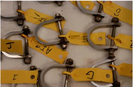
Previous work at Brigham Young University by Clark indicates that corrosion resistance of stainless steel can be improved by underwater friction stir welding as compared to fusion or arc welding [Clark, 2005]. Stainless steels are often used in applications where corrosion is a concern. Thus testing by Clark includes exposing the welded steel coupon to a boiling NaCl, saltwater, solution. This test is considered by Clark to be one of the best indicators of corrosion resistance due to the rigorous nature of the test. The test coupons are held in the U-bend configuration under tension when
exposed to the solution leading to a worst case corrosion scenario and a good test for underwater friction stir welding as a means to improve weld characteristics by virtue of
the advantages laid out by Mishra and Ma. U-bend samples can be seen in figure 12. The tension is kept by the bolt between the two ends of the coupon.
Figure 12: U-bend test samples prior to NaCl testing from Clark
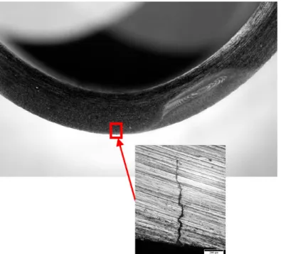
Results from Clark show that the advantages of underwater friction stir welding over fusion welding are obvious in the area of corrosion resistance. Fusion welds showed signs of root crack initiation after the solution test while UW-FSW’s did not show an initiation pattern of crack propagation in the weld zone. Evidence of this advancement is shown in below in figure 13.
Figure 13: Crack growth in the parent material in UWFSWed 304L SS (Clark, 2005)
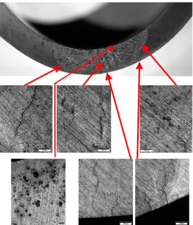
Cracks are much more readily observed for the fusion welds after the NaCl testing. Cracks did not simply initiate in one location, but were observed by Clark in many locations in the weld nugget. Pitting of the weld is also observed in the arc welded bend test. As Clark points out additional holes or discontinuities would only exacerbate the severity of the pitting in arc welds. Figure 14 shows the etched arc weld in the U-bend configuration after the boiling saltwater test for corrosion resistance.
Figure 14: Multiple crack initiation sites in the nugget from FSWed 304L SS (Clark, 2005)
Sakurada et al. rotary friction welded AA6061 rods in ambient air and
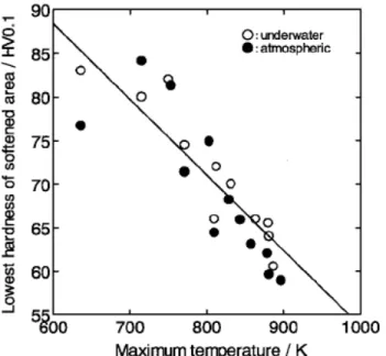
underwater. The study does a good job to illustrate best the mechanism for reduction of grain size in the current literature. Rotary friction welding involved rotating a metal rod at high speed and plunging it into another rod generating the heat proper to weld the two rods together. Parameters for SFW include rotation speed, shielding gas if welding ferric alloys, and plunge time before the rod is brought to a halt. The study observed many phenomena discussed in later chapters including the steep temperature gradients in submerged friction welding, SFW, as well as the increase in hardness of the weld zone which is coupled to the reduction of grain growth. As the maximum welding temperature is reduced, the hardness and subsequently the grain size of the nugget tend to drop linearly as seen below in figure 15 by Sakurada et al. Further observations included the
increase in UTS by the SFW’s over the conventional friction welds performed in ambient conditions. These can be seen in figure 16 which show an increase in rotary friction welded pipe ultimate tensile strength of approximately 4% when welded underwater.
Figure 15: Minimum hardness (HV) vs. Maximum T (K) for friction welded AA6061 (Sakurada et al., 2002)
It can be seen that both processes seem to indicate a linear decrease in hardness with maximum weld temperature rise. Welding processes, in air and underwater, increase nugget hardness with a lower maximum weld temperature, but the underwater welds generally outperform ambient welds for any constant temperature.
Figure 16: Joint efficiency (%) vs. welding time (s) for L) welds in air and R) underwater welds
Finally the study by Sakurada concludes by plotting the trend that the joint efficiency increases directly proportional as the hardness in the nugget increases in both ambient and underwater testing. This plot showed that a hardness increase in AA6061 from 60 to 90 HV (Vickers hardness) can lead to a joint efficiency increase of nearly 33%
in rotary friction welds and is observable in figure 17.
Figure 17: Joint efficiency (%) vs. Lowest hardness (HV) for underwater and atmospheric welds (Sakurada et al,. 2005)
CHAPTER III
EXPERIMENTAL PROCEDURE
All ambient air and underwater friction stir welding experiments were conducted using a Milwaukee #2K Universal Milling Machine modified with a Kearney and Treker Heavy Duty Vertical Head Attachment at Vanderbilt’s Welding Automation Laboratory.
The milling machine was modified in order to automate the welding process. This involved selecting pulley ratios suitable for welding at speeds or torques different than the initial configuration allowed. The experimental friction stir welding machine used at VUWAL is shown in figure 18.
Figure 18: FSW machine at VUWAL (Photo courtesy of Paul Sinclair)
The axial, or spindle, motor used in the Trivex probe experiment was a Baldor 20 hp 3-phase AC motor. The pulley ratio used in this study was 4:3 and was set in order to under drive the spindle to lower speeds and higher torque. The maximum speed allowed by the motor was approximately 2300 rpm at 60 Hz input. The pulley ratio for the
threaded probe experiment was 3:4 allowing a maximum spindle speed of 4500 rpm. The lateral and traversal motors were both U.S. Electric 1 hp motors with an in-line gear box ratio of 6.02:1. This leads to a reduction in maximum speed from 1750 to 280 rpm at 60 Hz, but an increase in maximum torque. The traversal motor had an additional 11:2 pulley ratio added to under drive the motor to a maximum allowable traverse speed of 16 ipm. Welding coupons were 1/4” thick, 8” long by 3” wide full penetration butt joints.
The tool in both experiments used a shoulder to pin diameter ratio of 2.5. Exact dimensions of the tool are shown in figure 19.
Figure 19: Tool dimensions in inches for both experiments (Probe not featured)
The probe used for the first experiment was a Trivex™ design by TWI
[Colegrove and Shercliff, 2003] noted for its decrease in welding forces with a static tool pin diameter of ¼” (6.35 mm). The second experiment used a threaded pin design with
¼” diameter and 20 threads per inch (tpi). The pin cross-section for the Trivex probe was developed by TWI as an equilateral triangle with sides given a specified convex radius.
The configuration used gives the tool probe static area to swept area ratio of
approximately 68%. This corresponds to the “a / Ra” ratio of 1, in which the center of the radius of the curvature is at a vertex of the triangle. The plot showing the Trivex area ratio as a function of the radius the side is below in figure 20.
Figure 20: Trivex parameters vs. area ratio (tool used has a ratio of .68)
Experimental results by TWI show that the Trivex tool welds were comparable to those of the more complex Triflute or Triflute-MX designs [Colegrove and Shercliff, 2003]. Tool profiles for Trivex and Triflute tools are given in figure 21. The shoulder diameter was 5/8” (15.875 mm) and featureless. The tool and probe for both experiments were machined from 01 tool steel and heat treated.
Figure 21: a) Triflute b) Triflute – MX c) Trivex probes from TWI (Colegrove and Shercliff, 2003)
During either experiment no visible wear or deformity was observed on the tool pin or shoulder. The tool angle and plunge depth was held constant in the Trivex probe experiment at 1º and .009” respectively. The angle and depth used for the threaded experiment was 2o and .004” respectively. These plunges were used so that there is an 80% shoulder contact condition desirable for welding.
A Kistler rotating cutting force dynamometer (RCD) Type 9123C was used to measure traversal force (Fx), lateral force (Fy), axial force (Fz), and tool moment (Mz).
The dynamometer was rated to measure up to 20kN of axial force and 200 Nm of torque.
Experimental force measurements for both IFSW and FSW were found to be well below the limits. The welding machine was fitted for position control using string
potentiometers for translational and lateral location tracking.
Small changes in vertical position cause significant changes in weld quality as well as excess flash or wormholes [Crawford et al., 2006]. The vertical axis was instrumented with a magnetic position transducer with quadrature output leading to position resolution on the order of < .0005” (.0127 mm).
Thermocouple Implantation
Welds in the Trivex tool probe study were implanted with type K, Al – OH, thermocouples to determine characteristic temperatures and quench rates into the medium whether it was air or water. It has been previously observed that the welding temperature at a lateral location was not greatly affected by the traversal distance [Hofmann and Vecchio, 2005] [Mitchell, 2002] [Elangovan and Balasubramanian, 2008]. Multiple thermocouples were imbedded to ensure an accurate temperature reading. Four equally spaced thermocouples were placed into each weld at a thickness of 1/8”, or half the thickness of the ¼” coupons, and a depth of 1.1875”. This corresponded to the lateral position of the shoulder edge during welding. The diameter of the thermocouple hole was .1 inches or the nominal thickness of the thermocouple itself. The hole was filled with a generous amount of colloidal silver thermal paste from SPI supplies in order to ensure contact and maximum conductivity. This layout is shown in figure 22.
Figure 22: Thermocouple hole dimensions (all units in inches)
Heat input into the water was important to verify certain process trends. It also served to quantify the power increase required to successfully produce IFSWs. A lower
limit for heat input was computed using the change in water temperature before and after welding. Heat input was measured for IFSW using the equation for single state enthalpy change.
T mc H = p∆
∆ (1)
Heat input is simply the change in enthalpy of a substance in a constant state where “m” is the mass of water, “Cp” is the specific heat at constant pressure, and “∆T”
is the change in water temperature before and after welding. This approach was applied to the SFSP conducted by Hofmann and Vecchio. This was ideal since the variation in water temperature was relative and not absolute and thus the water did not need to return to room temperature prior to welding again. Water for the experiment was initially room temperature (~298K) and kept at a constant volume of 3 L for all immersed welds. It should be noted that the enthalpy method does not assume a loss of heat due to
conduction through the backing plate or convection into the air at the surface. All that is measured is the amount of heat input into the water through the heating due to welding.
An additional heat input equation is given by Nunes [Schneider et al., 2006]
which gives the heat input during FSW. The heat input, ∆H, in energy per unit distance traveled is given as:
v P H = /
∆ (3)
Where ‘v’ is the travel speed (m/s) and ‘P’ is the power (J/s).
Zω M
P= (4)
Where ‘Mz‘ is the torque required to weld in Newton-meters and ‘ω’ is the rotational speed in Hertz (1/s). This heat input and power equation predicted accurate trends. The power estimation predicted an approximately constant power output for a range of spindle speeds. This was modeled and experimentally verified by Crawford et al.
where for a substantial increase in rotational speed a substantial decrease in torque followed [Crawford, 2006].
Experimental setup for threaded cylinder
The second setup for IFSW involved a different tool pin configuration and modified weld matrix. Runs were performed on the same welding machine and dynamometer. This was due to the expectation of similar forces and comparable
parameter matrices as the prior setup. The tooling used was a more conventional threaded cylinder and flat, featureless shoulder. Its advantages include imposing a strong
downward flow which is complimentary to the rotary flow around the pin [Schneider et al., 2006]. Together the two flows increase stirring, leading to a further breakdown of the oxide layer and greater root fill and mixing producing good welds. The tool pin and shoulder diameters were .25” and .625” respectively with a thread pitch of 20 threads per inch. The pin length of the non-consumable heat-treated 01 steel tool was .235”.
Properties of 0-1 heat treated tool steel are shown in Table 4.
Table 4: Composition of 0-1 oil hardened tool steel 0-1 tool
steel
Carbon, C
Chromium, Cr
Iron, Fe Manganese, Mn
Tungsten, W
Vanadium, V
% 0.90 0.50 97.0 1.0 0.50 0.15
Disadvantages of the threaded cylinder tool design include the lack of a significant dynamic volume greater than that of the static tool volume during welding which decreases mixing when compared to the Trivex profile. Secondly, the threaded cylinder produces higher traverse, moment, and forge (Fx, Fz, Mz) forces compared to the Trivex experiment’s tool. The Trivex design was made for this purpose by Colegrove and the threaded cylinder’s increased forces lead to a larger work envelope and fewer defects than a similar Trivex matrix. The work envelope for this experiment included rotation speeds (RS) of 2000-3000 rpm and travel speeds of 10-16 ipm (inches per minute). Tool tilt angle and plunge depth where kept constant for the all experimental welds at 2o and .004”.
Tank Construction
The backing plate, or backing anvil, was modified to contain approximately three liters of water for both experiments (see figure 23). The sides of the tank are ¼” clear acrylic and are mounted and sealed along the outside of the mobile backing anvil. The submergible anvil is placed on top of the standard FSW anvil on the welding machine.
The dimensions for the containment tank were 12 inches by 29.75 inches. Water was placed in the tank to a level of ½” deep using a graduated cylinder. This gave a total volume of approximately 178.5 cubic inches or 2.925L.
Figure 23: Tank containing water used for SFSW
CHAPTER IV
EXPERIMENTAL RESULTS AND CONCLUSIONS FOR THE THREADED PROBE TOOL
The test bed travel motor was set up to deliver between 0 – 16 ipm and the rotation speed was from 0 – 4500 rpm. This was accomplished by changing the gear pulley ratio. The threaded probe tool produced good welds in a range in spindle and travel speeds. The increases in force were the result of the vertical flow theorized by Schneider et al. which was increased by the threads on the probe. The Trivex’s advantage of mixing laterally, while advantageous, did not create defect free welds at most weld speeds as the threaded probe does.
Optimal welds were run under ambient conditions from previous research by Crawford et al. Optimal ‘dry’ welding conditions were found to be 2000 rpm at 16 ipm.
These welds were found to have minimal joint line defects and high ultimate tensile strength (UTS). Optimal welds for immersed conditions were determined by running a matrix which included rotational speeds of 2000, 2200, and 3000 rpm as well as travel speeds of 10, 15, and 16 ipm. Three tensile test coupons were cut from each weld to ensure the precision of the data. Test coupons were made to ASM specifications for tensile testing of a butt weld specimen. The geometry of the test coupon is shown in figure 24.
Figure 24: Tensile coupon schematic
The optimal welding conditions for IFSW were found to be 2000 rpm at 10 ipm.
This corresponded to the greatest weld tensile strength of either underwater or in air FSW. The weld pitch of the optimal weld was found to be 200 revolutions per inch (rpi) for this matrix. The worm hole defect was discovered by tensile testing and occurred on the advancing side of the submerged weld 3000 rpm at 15 ipm, also at a weld pitch of 200 rpi. This is a verification of the weld pitch section made in chapter II. The same weld pitch using different parameters gave bad weld quality in one of the two runs. All other welds were found satisfactory. They fractured outside of the weld nugget and TMAZ in the weld heat affected zone (HAZ), an area of lower hardness than both the nugget and parent material due to the lack of mixing and dynamic recrystallization. Welds from the threaded pin matrix are shown in figure 25. All specimens that are not labeled as FSW in the figure are IFSW runs.
Figure 25: Tensile specimens from the threaded probe matrix
Even with the void defect present at 3000 rpm and 15 ipm the tensile strength was 60% of the parent material UTS. This is good in comparison to ambient friction stir welds where weld quality is deteriorated by voids to below 50% or worse in fusion welding.
Data from the weld matrix run using the threaded probe is shown in table 5. It can be seen that the best underwater welds (designated WC#) performed as well as or better than control ambient air welds (designated BW#). Percent UTS of the parent material was found to be approximately 5% higher for IFSW than ambient FSW.
Table 5: Force and data from the threaded probe experiment
Improvement of weld properties comes at a cost of increased torque and power.
The torque for FSW is approximately 16 Nm while IFSW torque values are 18.5 Nm, this is an increase of less than 25%. This form of weld in-situ heat treatment by quenching the weld was beneficial to weld quality and the cost in power input is low. Weld pitch
increases illustrate the power increase. The more revolutions the tool makes in an inch increased the power , or heat input, into the joint. The optimal ambient run was found to be at 125 rpi while the immersed run was found to be at 200 rpi. The power increase was small when compared to the 2.5 Nm required torque increase to achieve improved weld quality.
CHAPTER V
EXPERIMENTAL RESULTS AND CONCLUSIONS FOR THE TRIVEX PROBE TOOL
The Trivex probe used rotational speeds between 1000 - 2000 rpm. This was due to the lower forces created by the Trivex tool as identified by previous experimental and simulation based studies by Colegrove and others [Colegrove and Shercliff, 2004]
[Maziarz, 2006]. Travel speeds were from 5 – 14 inches per minute leading to a weld pitch from 71.4 - 200 rpi. The weld matrix for the following experiment is in table 6.
Table 6: Weld matrix used for Trivex tool experiment
1000 rpm 1500 rpm 2000 rpm
5 ipm X X X
8 ipm X X X
11 ipm X X X
14 ipm X X X
Axial Force
Axial force was measured using a Kistler Rotating Cutting Force Dynamometer.
Welding was position controlled, not force controlled. Thus force trends were
experimentally verified to determine how they depend on process parameters. Data for ambient friction stir welding as well as IFSW using the Trivex pin tool showed expected trends in which an increased rotation speed/decreased force relation was evident. This trend was also observed by previous research and was further validated for both
processes, FSW and IFSW [Crawford et al., 2006] [Bloodworth et al., 2008]. Axial force was expected to behave inversely proportional to weld pitch. IFSW and ambient FSW
runs show that axial force was independent of either process. This is evident in figures 26a – 26c. The experimental setup at Vanderbilt Welding Automation Laboratory is currently set to maintain greater than 12kN (2698 lbf) of axial force. Force plots for 1000 rpm and 1500 rpm illustrate trends indicating an identical axial force value exists for either process at the same rotation or travel speed.
Figure 26a: Axial force (N) vs. Travel Speed (ipm) at 2000 RPM
Figure 26b: Axial force (N) vs. Travel Speed (ipm) at 1500 RPM
Figure 26c: Axial force (N) vs. Travel Speed (ipm) at 1000 RPM
. The axial force was found to be independent of the process at all parameter values for this data set. It has been observed that axial force is a quality indicator for
friction stir welds. An insufficient axial force indicates a lack of shoulder pressure and can indicate a lack of containment of the surface flash and/or voids.
Torque
Torque values were recorded to quantify the power requirements for IFSW over conventional FSW. It was expected that the torque would increase as some of the frictional heating would go into heating the water. Torque values recorded for 1500 rpm and 2000 rpm are given for both processes in figures 27a – 27b.
Figure 27a: Moment (Nm) vs. Travel Speed (ipm) at 1500 RPM
Figure 27b: Moment (Nm) vs. Travel Speed (ipm) at 2000 RPM
An increase in torque was visible from 5-14 IPM for IFSW over FSW. An increase of 2-5 Nm (1.5 - 3.7 lb-ft) was required and was found to be a highly parameter independent change in torque. This was in agreement with previous experiments using the threaded probe tool. The increased weld pitch/decreased torque relationship was observed for both processes [Crawford, 2006] [Bloodworth et al., 2008]. This trend had been observed in even greater weld pitches and the limit to this trend has not yet been identified. The torque increase requirement was less than 25%. This shows the same increase observed using the threaded probe tool.
Power
The increase in power was proportional to the increase in torque and rotational speed. Power increased linearly as a function of travel speed. This indicates a travel speed to moment relationship observed by other authors. From figure 28 it can be observed that
the welding machine outputs between 1-5 kW for FSW and IFSW. The observed increase in power by the IFSW process is approximately .5kW or 15-20%. Power is determined by the equation:
Zω M
P= (4)
Where ‘Mz’ is the torque in Nm and ‘w’ is the rotation speed of the tool in Hz.
Figure 28: Power (kW) vs. travel speed (IPM) at 2000 RPM
Optimal parameters were determined by two factors. These include weld joint line remnants and tensile strength. The heat input into the water was used to observe process trends. It also quantified the power increase required to IFSW AA6061. A lower limit for heat input was computed using the change in water temperature before and after welding.
Heat Input as a Function of Welding Process
Heat input was measured by implanting thermocouples. In figures 29 and 30, as travel speed is increased or spindle speed is decreased the heat input into the weld drops.
The increase of thermal energy in the water is a lower bound to the heat input as energy is also input into plastically working the weld material as loses due to conduction and convection.
Heat Input vs IPM
0 50 100 150 200 250
5 8 11 14
IPM
Heat Input (kJ)
1000 RPM 1500 RPM 2000 RPM
Figure 29: Heat Input vs IPM for IFSW
Heat input vs RPM
0 50 100 150 200 250
1000 1500 2000
RPM
Heat Input (kJ)
5 IPM 8 IPM 11 IPM
Figure 30: Heat Input vs RPM for IFSW
Materials Testing
Materials testing included micro-hardness analysis, cross-sectioning, and tensile testing of all welded specimens. Some parameters were not run for the immersed matrix since was determined that the rotational speed was not enough to produce welds at 14 IPM with the exception of 2000 rpm. The wormhole defect was prevalent in welds below 2000 rpm. Further welds were not run as it was assumed that the wormhole would only increase in size.
Tensile testing was performed on welds in order to determine optimal parameters.
Optimal runs were then used to compare micro-hardness using the weld cross section.
Hoffman and Vecchio observed an order of magnitude decrease in the weld nugget grain size over conventional friction stir processing (FSP) [Hofmann and Vecchio, 2005].
Micro-hardness tests performed on IFSW’s show an increase in local weld hardness over standard FSW. Microscopy indicated that optimal conditions retained the same root
properties. Although porosity was observed in optical microscopy of the weld zone, tensile properties matched or exceeded those of conventional friction stir welds.
Figure 31: Hardness (HV) vs. Weld Nugget Location (mm)
The increase in quench rate due to IFSW causes the grains to quench and solidify from its plastic state without excessive grain grown leading to a harder weld nugget.
Hardness testing indicated an approximately 10% increase in weld zone hardness. Weld zone hardness test results for this experiment showed an average weld nugget hardness of 73 for conventional FSW and 81 for IFSW (see figure 31). Hardness tests were
performed only on the highest tensile test welds for either process. These included welds which when cross sectioned showed no evidence of defects including worm holes or excess flash.
Cross sections were polished and etched using Boss’s reagent at 10:1 ratio of water to hydrofluoric acid (HF) for 15-20 seconds. Weld zone cross sections showed a smaller heat affected zone and joint line remnant for IFSW when compared to
conventional FSW. Figure 32 shows the porosity generated in the IFSW (right) is evident when compared to standard FSW (left).
Figure 32: L) Conventional FSW root flaw (10x) R) Immersed FSW root flaw (50x)
Tensile tests were run to determine the optimum weld parameters for both FSW and IFSW. Tests were conducted according to the ASM standard for materials testing.
Ultimate tensile strength (UTS) was the criterion for rating weld quality. Optimal welds had welded to parent material UTS ratio was greater than 75%. For the matrix given above, the optimal weld conditions for FSW were 2000 rpm at 11 ipm while the IFSW required 2000 rpm at 8 ipm, a decrease of 3 ipm. Variations in parameters from the threaded probe experiment were due to the probe changing to Trivex. This leads to an increase in power to show the same forces. The solution to the force decrease was a decrease in travel speed to improve mixing and vertical flow.
This is due to the power increase to form the bond. Heat flows into the water raising its temperature. Water has a heat capacity four times that of room temperature air.
It requires four times the heat input to heat an equal mass of water than that of air. It is observed that a decrease in travel speed is required to increase the heat input into IFSW’s.
For a constant travel speed (TS) it was observed that the weld quality increased with rotational speed (RS). This was observed mostly in FSW while IFSW seem to indicate a logarithmic trend with respect to RS for the matrix run. For each TS run (5, 8,
11 ipm) in the IFSW matrix the trend for tensile strength vs. RS remained a logarithmic function of RS. Figure 33 illustrates the logarithmic relationship between weld UTS vs.
RS at a constant TS. Results for a constant rotational speed showed independent UTS with increased TS.
The primary failure mode outside the optimal parameter envelope was the wormhole defect. This is caused by a “cold” weld without sufficient heating of the joint and therefore a lack of mixing causes a tunneling defect near the root of the weld. The threaded cylinder pin, as opposed to the Trivex™ tool used in this study, created greater downward flow and higher forces leading to a larger envelope for IFSW. Improvements in weld quality are made by IFSW of the joint. In-situ heat treatment in the form of quenching gives the joint a better UTS and weld nugget hardness.
Figure 33: UTS (MPa) vs. RS at a constant TS (IFSW); WA = 1000rpm, WB = 1500rpm, WC = 2000rpm
CHAPTER VI
FINITE ELEMENT MODEL OF STEADY STATE WELDING TEMPERATURE BASED ON FORCE DATA
In order for the wide spread application of FSW to be instituted, an overall understanding must be made as to the complex thermal and mechanical properties inherent and unique to this technique. Presented in this chapter is a steady state thermal model of a conventional FSW tool and tool pin. A steady state model is presented using Patran and Nastran along with a comparison to experimental runs run by the Vanderbilt University Welding Automation Laboratory (VUWAL). The results are discussed and compared to the experimental data gathered using a Mikron Thermal imaging Camera.
The purpose of the study is to understand the temperature distribution as a function of welding parameters. The verification of the model experimentally captured the
temperature distribution up the tool accurately. The influence of the shoulder and tool shank leading to serve as a heat sink is also discussed.
The welded material during FSW is brought to a temperature approximately 60- 80% of its melting point [Ulysse, 2007]. This increase in welding temperature decreases the yield strength of the material dramatically. The temperature dependent yield strength curve for AA6061-T6 used in the experimental stage is given in figure 34.
Yield strength vs. Temperature
0 50 100 150 200 250 300
250 350 450 550 650
Temperature (K)
Yield Strength (MPa)
sy (MPa)
Figure 34: Temperature dependent yield strength of welded AA6061
It is critical that the welding tool can support these kinds of temperatures without plastic deformation itself. Arthur Nunes of Marshall Space Flight Center has concluded that the yield strength of the welding tool at maximum temperature should have three times the yield strength of the welded material to be considered semi-infinite or non- consumable. A simulation which would accurately predict the heat generation due to the frictional interface between the tool shoulder and pin with the work piece is needed to develop an operational window for tools. Heat generation for the simple FSW tool and pin was presented by Schmidt et al. as an analytical model [Schmidt et al., 2004]. This model will be implemented in a three dimensional steady state thermal analysis of the welding process.
Background
Schmidt et al. developed an analytical model for the friction stir welding tool using a number of assumptions on the contact boundary condition. The simplest boundary condition to implement is a no-slip condition; this means that there is no movement of the weld material to the tool at the tool-weld interface. The heat generation
for the shoulder bottom, tool pin sides, and tool pin bottom are found using geometric sums of infinitesimal areas. The heat generation for the sticking condition used in the simulations of this work can be seen in equations 8-10.
) 10 3 (
2
) 9 ( 2
) 8 ( ) tan 1 )(
3 ( 2
3 2
3 3
pin c bottom
pin c sides
pin sh c shoulder
R Q
H R Q
R R Q
ω πτ
ω πτ
α ω
πτ
=
=
+
−
=
Where tc is the contact stress in Pa and w is the rotational speed in Hz. Rsh and Rpin are the shoulder and pin radius in meters respectively and a is the angle of the shoulder in radians. Upon further inspection one can see that the primary heat generation component is the shoulder, followed by the pin sides and bottom. Heat due to the
shoulder contributes approximately ¾ of the total heat generated by the tool. Another 1/5 is due to the sides of the pin, and the remainder is due to the pin bottom’s frictional interface. The yield strength, sy, of AA6061-T6 at 300K is 241E6 Pa [N/m2]. The dimensions for the FSW tool simulated and experimentally used are seen in figure 35.
Figure 35: Tool used in steady state model and experiment
The experimental tool had a so-called non-profiled shoulder with 00 included angles (a). The tool used in the experimental setup is H13 tool steel hardened to a Rockwell C-scale hardness of 48-50. Composition of H13 tool steel is shown the table 7.
Table 7: Elemental composition of H13 tool steel H13 tool
steel
Carbon, C
Silicon, Si
Manganese, MN
Chromium, Cr
Molybdenum, MO
Vanadium, V
% 0.40 1.10 0.40 5.30 1.40 1.00
Description of the Model
The finite element package Patran was used for the preprocessing of the data and Nastran was the solver used to find steady state solutions to the thermal model [Patran and Nastran, 2005]. The model consisted of 18360 3D elements (15260 CHEXA and 3100 CPENTA) and 18711 nodes. The solids were meshed using Hexagonal and
Pentagonal isometric meshing schemes (isomesh). The model used a total of 3 solids and 7 surfaces including the “donut” surface of the shoulder visible to the weld material. This
was created by breaking the original circle into two surfaces at the interface of the pin and shoulder. This surface was critical as only the visible shoulder contributes to heat generation, not the shoulder “covered” by the pin. An isometric view of the finite element mesh is seen in figure 36. A verification of the mesh and further details are in the
appendix.
Figure 36: Isometric view of finite element mesh
The thermal conductivity of the tool was set to 202 W/ (m*K) corresponding to H13 properties. Boundary conditions matched observed conditions for experimental runs. The tool shank was set to a constant 298K ambient air temperature at the top surface of the 3 inch tool. This includes the outer surface from 1 inch and above. This models the solid interface between the tool and the vertical head which serves as a large heat sink. For simplicity all units in figure 35 are converted to meters in the finite element model. The boundary conditions on the tool shank are displayed in figure 37.
Figure 37: Boundary conditions for the tool used in the FEA
Heat generation (W/m2) from the tool shoulder, pin sides, and pin bottom are solved used the above analytical model, multiplied by the respective areas of influence to create a total load. The loads are then applied to their respective surfaces. A sample loading can be seen in figure 38.
Figure 38: Load values for a FE simulation for steady state heat generation
The values used for heat generation, Q, are available in appendix C. Rotational speeds for the spindle are traditionally given in literature as revolutions per minute (RPM), however, the rotational frequency in the heat generation terms require Hertz (radians/sec). Rotational speeds of 1500-4000 rpm’s were experimentally run and used to validate the simulations. The main variable parameter, rotational speed, of 1500-4000 rpm’s corresponds to 157-419 Hz (rpm*2p/60=Hz), a unit necessary for the analytical model by Schmidt et al.
Results and Comparisons
Simulations were run on a Toshiba Satellite Laptop with Intel Centrino Duo processor working at 1.66 GHz and 1 GB RAM. Run time for the Nastran solver took
~.31 seconds dependent on the parameters used. As expected from the analytic model, tool motion across the weld line is not modeled (i.e. translational speed). This leads to an axisymmetric model. An axisymmetric model should give identical results to the 3D analysis although findings are not submitted here. The welding tool as seen in the Trivex study and other posed in the literature does not greatly increase the welding temperature as it traverses the weld [Hofmann and Vecchio, 2006] [Mitchell, 2002]. Thermocouples tend to read the same temperature at any distance along the weld path at a specified distance from the centerline. Temperature isotherms for w = 1500 and 3500 rpm’s can be seen in figure 39. The welding temperature, Tw, is defined as the maximum temperature along the primary contact surfaces (i.e. shoulder and pin side). Simulations run at w = 1500 give a welding temperature of 564K (2910C). For the 3500 rpm simulation Tw = 742K (4690C). Additional temperature graphs are available in the appendix.
![Figure 1: Schematic of the Friction Stir Welding Process [Mishra and Ma, 2005]](https://thumb-ap.123doks.com/thumbv2/123dok/10741018.0/11.918.255.718.576.831/figure-schematic-friction-stir-welding-process-mishra-2005.webp)