8
Process experimentation with two or more factors
Many important phenomena depend, not on the operation of a single factor, but on the bringing together of two or sometimes more factors at the appropriate levels. (Box, 1990, p. 365)
Overview
The design of experiments (DOE) is a vast topic – designed experiments are major tools for use in the improve phase of many Six Sigma projects. In the previous chapter experiments involving only a single factor of interest were considered. In this chapter experiments involving two or more factors of interest will be introduced. Much process improvement experimentation is done on a one-factor-at-a-time basis. Although such experimentation can lead to improvement, there is no doubt that multifactor experiments, in which factor levels are varied systematically according to a recognized design, can be much more informative.
In particular, multifactor experiments can reveal the presence of important interactions between factors. Harnessing interaction effects can lead to dramatic process improvements.
Minitab can be of assistance both with the actual design of the experiment and with the display and analysis of the resulting data. Following a general introduction, in which the concept of interaction will be introduced, experiments in the 2kseries, withkfactors, each with two levels, will be considered. Screening experiments and fractional factorial experiments in the 2k p series will be introduced, together with the concept of design resolution. The fundamentals of response surfaces will be described. Reference will be made to Taguchi experimental designs.
Six Sigma Quality Improvement with Minitab, Second Edition. G. Robin Henderson.
2011 John Wiley & Sons, Ltd. Published 2011 by John Wiley & Sons, Ltd.
8.1 General factorial experiments
8.1.1 Creation of a general factorial experimental design
As an introductory example, consider the process of making popcorn. Two factors are of interest – the first is the type of popper (X1) and the second is the grade of corn used (X2).
The levels of interest for popper are air and oil, those for corn are budget, regular and luxury.
The response of interest is the volume (ml) yield of popcorn (Y) from 250 ml of corn processed according to the instructions provided by the manufacturers of the machines. The design may be created usingStat>DOE>Factorial>Create Factorial Design. . .for which the initial dialog is shown in Figure 8.1.
The first step is to select General full factorial design withNumber of factors: 2 specified. (With the generality of this type of design it is not possible to provide a catalogue of designs underDisplay Available Designs. . ..) The second step is to click onDesigns. . .and engage in the subdialog as indicated in Figure 8.2.
The name of each factor may be entered together with the number of levels – in this case popper has two levels and corn has three. The defaultNumber of Replicates:is 1, but in this experiment 4 was the number used. This means that the process was operated four times with each of the 2 (levels of popper)3 (levels of corn)¼6 factor-level combinations (FLCs) – we say that it wasreplicatedfour times. Thus the term ‘replicate’ is being used in a technical statistical sense in the context of designed experimentation. (When more than one replicate is employed the opportunity to block on replicates is made available but was not required in this case.) Having clicked OK, click on Factors. . . and complete the dialog shown in Figure 8.3. Here the categorical levels for the factors mean thatTypeshould be selected as Text. (Numeric would be selected in the case of a factor such as temperature specified in degrees Celsius.)
UnderOptions. . .the default toRandomize runsis strongly advised as part of good experimental design practice. (If the user enters an integer underBase for random data generator:then subsequent use ofRandomize runswithCreate Factorial Designsand the
Figure 8.1 Initial dialog for general full factorial design.
same numbers of factors and levels and the same base leads to the same run order.) Opting to Store design in worksheet, which should of course be saved, is essential if data from the experiment are to be readily analysed later.
Having clicked OK and then OK again the design worksheet is created. The version obtained by the author is shown in Figure 8.4. It was augmented through the addition of a column named Yield for the recording of the yield obtained from each run and a column named Remarks in which those carrying out the experiment may note any unusual occurrences etc.
It also has a column of residuals and a column of fitted values obtained during analysis of the data following completion of the experiment.
The columns created by Minitab are as follows:
. a column showing the standard order for each run – the reader is invited to create the worksheet again with the Randomize runs option unchecked and to scrutinize the systematic pattern in the standard order column;
. a column showing the actual run order created by the randomization procedure;
Figure 8.2 Specifying the factors.
Figure 8.3 Specifying the factors: name, type, number of levels and level values.
GENERAL FACTORIAL EXPERIMENTS 305
. a column indicating point type in what is known as the design space – an explanation will be given later in the chapter (here all points are of type 1);
. a column indicating block – when there is no actual blocking this column consists entirely of 1s.
Armed with a copy of the worksheet, with the additional columns for yield and remarks added, the experimenters could head for the kitchen. The first run would have been with the air popper using 250 ml of luxury grade corn and would have given a yield of 1360 ml of popped corn, the second run would have been with the oil popper using 250 ml of luxury grade corn and would have given a yield of 1349 ml of popped corn and so on. Once the experimental work is complete display and analysis of the data can begin. The first eight columns displayed in Figure 8.4 are provided in worksheet Popcorn.MTW. The columns of residuals and fitted values in Figure 8.4 will be referred to later in the chapter.
8.1.2 Display and analysis of data from a general factorial experiment
The data may be presented in the form of a two-way table (Table 8.1) with rows corresponding to the levels of the popper factor and with columns corresponding to the levels of the corn factor. Each cell in the table gives the four replicate yields obtained with one particular FLC for the factors popper and corn. The mean yield for each cell is displayed in Table 8.2 together with the means corresponding to the rows (levels of popper) and columns (levels of corn) and the overall mean yield for the experiment.
Two forms of data display of these means are invaluable when dealing with data from experiments involving two or more factors – main effects plots and interaction plots. Use Stat>ANOVA>Main Effects Plot. . .to create the main effects plot; enter Yield under Reponses:and Popper and Corn underFactors:. The plot is shown in Figure 8.5.
The horizontal reference line indicates the overall mean yield for the experiment of 1214.7.
The mean yields for each of the two levels of popper are plotted in the first panel and the mean yields for each of the three levels of corn are plotted in the second. Two insights are obtained.
The first is that, on average, switching from the air popper to the oil popper reduces yield by Figure 8.4 Design worksheet with yields, remarks, residuals and fits from additive model.
about 200 ml. The second is that, on average, yield progressively increases as we switch from budget grade corn to regular to luxury.
Use Stat>ANOVA>Interactions Plot. . .to create the interactions plot; enter Yield underReponses:and Popper and Corn underFactors:. The plot is shown in Figure 8.6.
In this plot the six means at the core (shaded) of Table 8.2, each of which corresponds to an FLC, are displayed. The levels of corn are indicated on the horizontal axis. The levels of popper (see the legend in the top right-hand corner of the display) are indicated through the connection by line segments of those points that have the same level of popper. The pairs of line segments Table 8.1 Raw data for popcorn experiment.
Yield Budget Regular Luxury
Air 1120 1090 1360
1066 1342 1518
1106 1537 1585
1198 1260 1449
Oil 943 1289 1349
948 887 1108
923 1148 1241
1164 1058 1464
Table 8.2 Means summary of yield.
Mean Yield Budget Regular Luxury Mean
Air 1122.5 1307.3 1478.0 1302.6
Oil 994.5 1095.5 1290.5 1126.8
Mean 1058.5 1201.4 1384.3 1214.7
Figure 8.5 Main effects plot for popcorn experiment.
GENERAL FACTORIAL EXPERIMENTS 307
lying vertically above each other are approximately parallel. This means that, when using one particular grade of corn, similar decreases in mean yield are experienced on changing from the level air to the level oil of popper. This is characteristic of a situation in which there is no interaction between factors.
To create an alternative version of the interactions plot enter Yield underReponses:and Corn and Popper underFactors:i.e. reverse the order in which the factors are entered. The plot is shown in Figure 8.7. The levels of popper are indicated on the horizontal axis. The levels of the factor corn are indicated through connection by line segments of those points that have the same level of corn, as indicated by the legend. Again the segments lying vertically above and
Figure 8.6 Interaction plot – first version.
Figure 8.7 Interaction plot – second version.
below each other are approximately parallel. This means that, on changing the level of corn, similar changes in mean yield will be experienced, whether one is using an air popper or an oil popper.
If desired, both versions of the interaction plot may be created simultaneously by checking Display full interaction plot matrixin the dialog.
The data may be examined formally for evidence of interaction between the factors popper and corn by performing a two-way analysis of variance viaStat>ANOVA>Two-Way. . ..
The terminology ‘two-way’ relates to the presentation of data from a general factorial experiment involving two factors in the form of a two-way table, as in Table 8.1. The dialog is shown in Figure 8.8.
Note carefully that the Fit additive modeloption must not be checked as we wish to formally assess the evidence for the presence of interaction. UnderGraphs. . .it is strongly recommended that either theIndividual value plotorBoxplots of datadisplay be selected – when the number of replications is small the author recommends that the first of these plots be used. The Four in one option for Residual Plots is appropriate in this case since the observations of yield in the experiment are recorded in the worksheet in the time order in which they were obtained. The individual value plot is shown in Figure 8.9.
Note that the individual value plot in Figure 8.9 may be viewed as an ‘exploded’ version of the interactions plot in Figure 8.6 in which the individual yield values are plotted in addition to the yield means. The reader is invited to change the ordering of the factors in the dialog displayed on Figure 8.8 and to compare the individual value plot that is obtained with the interactions plot displayed in Figure 8.7.
As with the main effects plot in Figure 8.5 and the interaction plots in Figures 8.6 and 8.7, the plot in Figure 8.9 gives similar insights. It appears that:
. on average, switching from the air popper to the oil popper reduces yield by about 200 ml;
. on average, yield progressively increases as we switch from budget grade corn to regular to luxury.
Figure 8.8 Dialog for two-way ANOVA.
GENERAL FACTORIAL EXPERIMENTS 309
The standard residual plots are shown in Figure 8.10. The normal probability plot of the residuals is reasonably straight. Thus the assumption of a normal distribution of yield, for each combination of factor levels, is supported. Support for the assumption of a common variance for the distributions of yield for the six FLCs is provided by the similar vertical spread in all six groups of points in the plot of residuals versus fitted values. We can therefore proceed to interpret the ANOVA table with confidence that the assumptions underlying the valid application of theF-tests are reasonable.
Figure 8.9 Individual value plot of yield data.
Figure 8.10 Residual plots.
The ANOVA table is shown in Panel 8.1. In total we have a sample of 24 values of yield from the experiment so there are 24 1¼23 degrees of freedom (DF) in total. With 2 levels of popper there is 2 1¼1 degree of freedom for popper, and similarly 3 – 1¼2 degrees of freedom for corn. The number of degrees of freedom for the interaction between popper and corn is the product of the numbers of degrees of freedom for these two factors, i.e. 12¼2.
Thus the number of degrees of freedom for error is obtained by calculating 23 (1 þ2 þ 2)¼18. The sums of squares (SS) are calculated using formulae that need not concern us; the mean squares (MS) are obtained by dividing each SS by its corresponding DF. Provided the assumptions referred to above are valid, the ratios of the MS values for popper, corn and interaction will haveF-distributions. These enable the calculation ofP-values.
The experiment provides no evidence of interaction between popper and corn since the P-value for interaction of 0.820 is well in excess of 0.05. This means that there is no evidence from the experiment that the effect on yield of changing the grade of corn used depends on the type of popper being used. When there is no evidence of interaction in a two-factor experiment of this nature one can proceed to fit an additive model. This may readily be achieved usingEdit Last Dialog and checking Fit additive model. In addition Store residualsandStore fitswere checked in order that fitted values and residuals were available for explanation that follows. These fitted values and residuals are displayed in the columns labelled RESI1 and FITS1 in Figure 8.4. The residual plots were again satisfactory (but are not displayed here) and the revised ANOVA table is shown Panel 8.2.
For popper theP-value is 0.004 so this means that the main effect of popper is significant at the 1% level. The main effect of corn is significant at the 0.1% level. Thus the experiment provides strong evidence that the factors of interest – type of popper (X1) and grade of corn used (X2) – influence the response of interest, i.e. the volume (ml) yield of popcorn (Y), from 250 ml of corn processed according to the instructions provided by the manufacturers of the machines.
We will now introduce and fit the formal additive model underlying the analysis. Reference to Table 8.2 enables the effects for popper to be calculated as indicated in Table 8.3. The overall
Two-way ANOVA: Yield versus Corn, Popper
Source DF SS MS F P Corn 2 426586 213293 11.51 0.001 Popper 1 185328 185328 10.01 0.005 Interaction 2 7428 3714 0.20 0.820 Error 18 333423 18523
Total 23 952765
S = 136.1 R-Sq = 65.00% R-Sq(adj) = 55.28%
Panel 8.1 ANOVA for model with interaction.
Two-way ANOVA: Yield versus Corn, Popper
Source DF SS MS F P Corn 2 426586 213293 12.52 0.000 Popper 1 185328 185328 10.87 0.004 Error 20 340851 17043
Total 23 952765
S = 130.5 R-Sq = 64.23% R-Sq(adj) = 58.86%
Panel 8.2 ANOVA for additive model.
GENERAL FACTORIAL EXPERIMENTS 311
mean yield for the experiment was 1214.7 ml. The effect corresponding to a particular level of a factor is the mean yield for that factor level minus the overall mean yield for the experiment. Hence the air popper effect is 1302.6 1214.7¼87.9 and the oil popper effect is 1126.8 – 1214.7¼ 87.9. Thus we can interpret the effect of using the air popper as being to elevate yield from the overall mean of 1214.7 by 87.9 ml on average, and the effect of using the oil popper as being to depress (because of the negative effect) yield by 87.9 ml on average. Note that the two effects sum to 0.
Reference to Table 8.2 enables the effects for corn to be calculated as indicated in Table 8.4, and the reader is invited to confirm the calculations. Thus we can interpret the effect of using the budget grade corn as being to depress yield from the overall mean of 1214.7 by 156.2 ml on average, that of using the regular grade being to depress yield by 13.3 ml on average and that of using the luxury grade being to elevate yield by 169.6 ml on average. Note that the three effects sum to 0 (allowing for rounding of the means quoted in Table 8.2 to one decimal place).
The reader will recall from the previous chapter that
Observed data value¼Value fitted by modelþResidual;
which we abbreviated as
Data¼FitþResidual:
In this case we take
Fit¼Overall meanþPopper effectþCorn effect:
The first experimental run was carried out using an air popper with luxury grade corn and gave a yield of 1360 (see Figure 8.4). The fitted value is given by
Fit¼Overall meanþAir popper effectþLuxury grade of corn effect
¼1214:7þ87:9þ169:6¼1472:2:
Thus the corresponding residual may be obtained as
Residual¼Data Fit¼1360 1472:2¼ 112:2:
Table 8.3 Effects for popper.
Level Mean yield Effect
Air 1302.6 87.9
Oil 1126.8 87.9
Table 8.4 Effects for corn.
Corn
Level Budget Regular Luxury
Mean yield 1058.5 1201.4 1384.3
Effect 156.2 13.3 169.6
Scrutiny of the column of residuals computed by Minitab (see Figure 8.4) reveals a value of 112.125. Again the small discrepancy is due to rounding. The reader is invited to calculate the next few residuals in order to check his/her understanding.
8.1.3 The fixed effects model, comparisons
Thefixedeffects model for a general two-factor design,with no interaction, is specified in Box 8.1. The number of levels of the row factor isa, the number of levels of the column factor is band the number of replications isn. For example, withi¼2,j¼3 andk¼1 we have the specific relationship
Y231¼mþa2þb3þe231:
For the popcorn experiment this states that the yield from the first run (k¼1, indicating the first replicate) with the oil type of popper (i¼2, indicating the second level of the factor popper) and the luxury grade of corn (j¼3, indicating the third level of the factor corn) is made up of the overall mean plus the effect of oil type of popper plus the effect of luxury grade corn plus a random error. Earlier we estimated the overall mean,m, as 1214.7, the effect of oil type popper,a2, as 87.9 and the effect of luxury grade corn,b3, as 169.6. Thus the fitted value for the combination of oil type of popper with luxury corn is the sum 1214.7þ( 87.9) þ169.6
¼1296.4. The values¼130.5, which is given beneath the ANOVA table and is the square root of the error MS in the ANOVA table in Panel 8.2, provides an estimate of the standard deviation sof the random error component of the model. The model predicts that the population of yields obtained that would be obtained with the combination of oil type of popper and luxury grade corn would be normally distributed with mean 1296.4 and standard deviation 130.5. Similar statements may be made about the other FLCs.
Follow-up comparisons are available viaStat>ANOVA>General Linear Model. . ..
The dialog is shown in Figure 8.11. InModel:we are communicating to Minitab the nature of the model we are using, i.e. Yijk¼mþaiþbjþeijk. Such models always include an overall mean and the random error term, so by entering Popper and Corn inModel:we are indicating the aiþbj terms in the core of the model. In the Comparisons. . . subdialog, Pairwise comparisons were selected, by the Tukey method. Grouping information andConfidence intervalwere both checked, with the default percentageConfidence level:
95.0 used. Part of the corresponding section of the Session window output is shown in Panel 8.3.
Observed data value¼Overall meanþRow factor effectþColumn factor effect þRandom error
Yijk¼mþaiþbjþeijk; i¼1;2;. . .;a; j¼1;2;. . .;b; k¼1;2;. . .;n Xa
i¼1
ai¼0; Xb
j¼1
bj¼0; eijkNð0;s2Þ
Box 8.1 Additive fixed effects model for two factors.
GENERAL FACTORIAL EXPERIMENTS 313
The interpretation, with rounding of values, is as follows:
. On average the yield with the oil type popper is 176 ml lower than that with the air type popper, with confidence interval 65 ml to 287 ml (to the nearest integer).
. On average the yield with regular grade corn is 143 ml higher than with budget grade corn, with confidence interval 22 to 308 ml (to the nearest integer).
. On average the yield with luxury grade corn is 326 ml higher than with budget grade corn, with confidence interval 161 to 491 ml (to the nearest integer).
. On average the yield with luxury grade corn is 183 ml higher than with regular grade corn, with confidence interval 18 to 348 ml (to the nearest integer).
Since the second confidence interval includes 0, we have no evidence that the mean yield with budget grade corn differs significantly from that with regular grade corn. The other confidence intervals provide evidence of the superiority in terms of yield of an air popper with luxury grade corn. The reader may, of course, arrive at the key conclusions by scrutinizing the grouping information provided in the Session window output prior to each set of confidence intervals.
If the aim is to maximize yield (Y) using a combination of the fixed set of levels of the factors popper (X1) and corn grade (X2) considered, the levels air and luxury should be selected.
There are indications of a clear ‘winning combination’ in this scenario. Note that this combination corresponds to selection of the level for popper corresponding to the greatest mean for the levels of popper and to the selection of the level for corn corresponding to the
Figure 8.11 General Linear Model dialog.
greatest mean for the levels of corn – see the main effects plot in Figure 8.5. However, it should be borne in mind that other responses might be used in decision-making, such as flavour and costs. It is also important to be aware that, when there are significant interaction effects, this pick-a-winner approach can lead to selection of an FLC that is not optimal.
As a second example, consider a hypothetical experiment performed by an internet retailer prior to the launch of new laptop computer on the market. The retailer manages its database of customers in homogeneous marketing groups of approximately 5000 customers. The factors of interest were price (X1), with levels £499, £549 and £599, and offer (X2), with levels software and wireless, and the response was number of sales (Y). Two replications were made of the full 32 factorial (the shorthand 32 indicating that the first factor has three levels and the second factor has two levels.) Thus each customer in two groups selected at random was sent an
Grouping Information Using Tukey Method and 95.0% Confidence Popper N Mean Grouping
Air 12 1302.6 A Oil 12 1126.8 B
Means that do not share a letter are significantly different.
Tukey 95.0% Simultaneous Confidence Intervals Response Variable Yield
All Pairwise Comparisons among Levels of Popper Popper = Air subtracted from:
Popper Lower Center Upper ---+---+---+---+
Oil -286.9 -175.8 -64.58 (---*---)
---+---+---+---+
-240 -160 -80 0
Grouping Information Using Tukey Method and 95.0% Confidence Corn N Mean Grouping
Luxury 8 1384.2 A Regular 8 1201.4 B Budget 8 1058.5 B
Means that do not share a letter are significantly different.
Tukey 95.0% Simultaneous Confidence Intervals Response Variable Yield
All Pairwise Comparisons among Levels of Corn Corn = Budget subtracted from:
Corn Lower Center Upper -+---+---+---+--- Regular -22.36 142.9 308.1 (---*---)
Luxury 160.51 325.8 491.0 (---*---) -+---+---+---+--- 0 150 300 450
Corn = Regular subtracted from:
Corn Lower Center Upper -+---+---+---+--- Luxury 17.64 182.9 348.1 (---*---)
-+---+---+---+--- 0 150 300 450
Panel 8.3 Session window output of comparisons.
GENERAL FACTORIAL EXPERIMENTS 315
e-mail inviting purchase of the new laptop for price £449 with the offer of free software.
Customers in a second pair of groups selected at random received the offer of the new laptop for price £449 with the offer of a free wireless networking module, and so on. The data, displayed in Table 8.5, are available in the worksheet Marketing.MTW.
An individual values plot of the data is shown in Figure 8.12. The plot was obtained via Stat>ANOVA>Two-Way. . . and Graphs. . . with Individual value plot selected. Fit additive modelwas left unchecked and the ANOVA table shown in Panel 8.4 obtained.
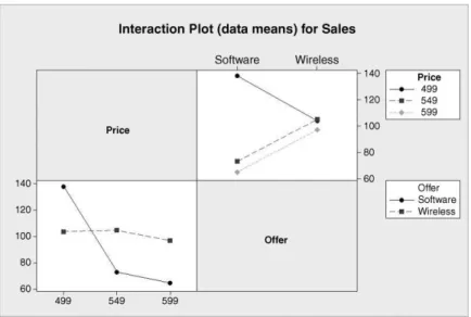
There is evidence of interaction in this case, withP-value 0.001. In such cases emphasis is put on understanding the nature of the interaction rather than on interpretation of the main effects. Use was made ofStat>ANOVA>Interactions Plot. . .with the optionDisplay full interaction plot matrixchecked to create the interaction plots shown in Figure 8.13. Unlike the previous example the vertical bands of line segments are far from parallel in some cases.
(In fact there is a crossing over in one case.) This is typical in situations where there is significant interaction between factors. There is evidence here that the effect on sales of changing the nature of the offer, from one of free software to one of a free wireless networking
Table 8.5 Data for marketing experiment.
Sales Offer
Price Software Wireless
£499 136 98
140 110
£549 72 96
74 114
£599 69 102
61 92
Figure 8.12 Individual value plot of marketing data.
module, depends on the level of price. For example, with price set at £499 there was a greater level of sales with the offer of software than with the offer of wireless, while at price £549 the opposite was the case. Having found evidence of a significant interaction effect the additive model fitted in the previous example will not be adequate.
Table 8.6 gives the mean sales corresponding to each of the 32¼6 FLCs. The Overall Mean Sales for the experiment was 97 laptops per group.
Table 8.7 gives the main effects for the offer factor. Note that the effects sum to zero.
Table 8.8 gives the main effects for the price factor. Note that the effects sum to zero.
As before, we have
Data¼FitþResidual:
In this case we take
Fit¼Overall meanþPrice effectþOffer effectþInteraction effect:
The interaction effect is obtained by computing, for each FLC, the value of Overall meanþPrice effect þOffer effect and choosing the interaction effect to be such that the fit
Two-way ANOVA: Sales versus Price, Offer
Source DF SS MS F P Price 2 3584 1792.00 32.98 0.001 Offer 1 300 300.00 5.52 0.057 Interaction 2 2904 1452.00 26.72 0.001 Error 6 326 54.33
Total 11 7114
S = 7.371 R-Sq = 95.42% R-Sq(adj) = 91.60%
Panel 8.4 ANOVA for marketing experiment.
Figure 8.13 Interaction plots of marketing data.
GENERAL FACTORIAL EXPERIMENTS 317
equals the mean sales in the experiment for the corresponding FLC. The detail is set out in Table 8.9. Note the mathematical symbols between the component sub-tables – the corre- sponding cell entries in the first four sub-tables are added together to give the corresponding cell entries in the final table.
For example, with level £499 for price and level software for offer, the sum of overall mean, price effect and offer effect equals 97þ24þ( 5)¼116. To obtain the mean sales figure of 138 for this FLC requires addition of a price–offer interaction effect of 22. With level £499 for price and level wireless for offer, the sum of overall mean, price effect and offer effect equals 97þ24þ5¼126. To obtain the mean sales figure of 104 for this combination of factor levels requires addition of a price–offer interaction effect of 22. The reader is invited to check the remaining entries in the fourth sub-table of Table 8.9. Note thatboththe rowsandthe columns of the matrix of interaction effects sum to 0.
Residuals are calculated as usual using Residual¼Data Fit. With price £499 and offer of software the two observed sales figures were 136 and 140, so the corresponding residuals are 136 138¼ 2 and 140 138¼2. (Whenever there are just two replications the residuals for each FLC will be equal in magnitude and opposite in sign.)
Thefixedeffects model for a general two-factor designwith interactionmay be specified as shown in Box 8.2. The number of levels of the row factor isa, the number of levels of the column factor isband the number of replications isn. For example, withi¼1,j¼2 andk¼3 we have the specific relationship
Y123¼mþa1þb2þ ðabÞ12þe123: Table 8.6 Mean sales for marketing experiment.
Offer Price
Software Wireless
£499 138 104
£549 73 105
£599 65 97
Table 8.7 Effects for offer.
Level Mean sales Effect
Software 92 5
Wireless 102 5
Table 8.8 Effects for price.
Level Mean sales Effect
£499 121 24
£549 89 8
£599 81 16
Table 8.9 Fitting the model.
Overall mean Offer
Price Software Wireless
£499 97 97
£549 97 97
£599 97 97
þ
Price effect Offer
Price Software Wireless
£499 24 24
£549 8 8
£599 16 16
þ
Offer effect Offer
Price Software Wireless
£499 5 5
£549 5 5
£599 5 5
þ
Interaction effect Offer
Price Software Wireless
£499 22 22
£549 11 11
£599 11 11
¼
Cell mean/fitted value Offer
Price Software Wireless
£499 138 104
£549 73 105
£599 65 97
Observed data value¼Overall meanþRow factor effect
þColumn factor effectþInteraction effectþRandom error Yijk¼mþaiþbjþ ðabÞijþeijk; i¼1;2;. . .;a; j¼1;2;. . .;b; k¼1;2;. . .;n Xa
i¼1
ai¼0; Xb
i¼1
bi¼0; Xb
j¼1
ðabÞij¼0; Xa
i¼1
ðabÞij¼0; eijkNð0;s2Þ
Box 8.2 Fixed-effect model for two factors with interaction.
GENERAL FACTORIAL EXPERIMENTS 319
For the marketing experiment this states that the sales to the third group (k¼3, indicating the third replicate) with price £499 (i¼1, indicating the first level of the price factor) and with the offer of a wireless module (j¼2, indicating the second level of the offer factor) is made up of the overall mean plus the effect of price £499 plus the effect of the offer of wireless plus the interaction effect for level £499 of the price factor coupled with level wireless for the offer factor plus the random error component. Earlier we estimated the overall mean as 97, the effect of price £499 as 24, the effect of offer wireless as 5 and the interaction effect, (ab)12, for this combination of factor levels, as 22. Thus the fitted value for the combination of price £599 with offer wireless is the sum 97þ24þ5 þ( 22)¼104.
The values¼7.371, which is given beneath the ANOVA table and is the square root of the error MS in the ANOVA table, provides an estimate of the standard deviationsof the random error component of the model. The model predicts that the population of sales to groups obtained with the combination of price £499 with the wireless offer will be normally distributed with mean 104 and standard deviation 7.371. Similar statements may be made about the five other FLCs.
The response, sales, is a discrete random variable so, strictly speaking, cannot be normally distributed for a particular combination of factor levels. However, a normal probability plot of the residuals is satisfactory so one can be satisfied that the assumption of normality, underlying the valid use of theF-distribution to computeP-values, is approximately true. The plot of residuals against fits is shown in Figure 8.14.
The symmetry of the plot about the horizontal reference line, corresponding to residual value 0, stems from the fact noted earlier that, with two replications, the residuals occur in pairs of values with equal magnitude. The reader might feel that the wide variation in spread of the pairs of points might cast doubt on the model assumption of a random error with constant variance. However, use ofStat>ANOVA>Test for Equal Variances. . .withResponse:
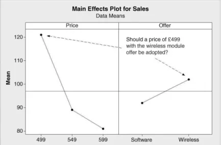
Sales andFactors:Price Offer, yields aP-value of 0.668. Thus there is no evidence from Bartlett’s test to cast doubt on a random error with constant variance. The main effects plot is shown in Figure 8.15.
Figure 8.14 Plot of residuals against fits.
In the case of the popcorn experiment, the best combination of factor levels, in terms of maximizing yield, could be identified by selecting the levels air and luxury on scrutiny of the main effects plot in Figure 8.5 for the levels of the factors corresponding to the greatest mean yields in each panel. In the case of the marketing experiment, scrutiny of the plot in Figure 8.15 might suggest the combination of price £499 with offer of wireless would be best, but, because of the interaction, it would appear that the combination of price £499 and offer of software is actually best – see Figure 8.12 and Table 8.6.
Grouping information from follow-up comparisons via the Tukey method with overall confidence level of 95% was obtained viaStat>ANOVA>General Linear Model. . .. The dialog is shown in Figure 8.16. InModel:we are communicating to Minitab the nature of the model we are using, i.e.Yijk¼mþaiþbjþ ðabÞijþeijk. By entering Price, Offer and PriceOffer inModel:we are indicating theaiþbjþ ðabÞijterms at the core of the model. In the Comparisonssubdialog Pairwise comparisonswere selected, by theTukeymethod.
Grouping information, withConfidence level:95.0 was checked. In theTerms:window PriceOffer was entered as interest centres on sales from the different FLCs, i.e. price–offer combinations. Part of the corresponding section of the Session window output is shown Panel 8.5.
Note that the FLC of price £499 and software offer ‘tops the league’ with the highest observed mean sales of 138. This FLC comprises grouping A, and as this letter is not shared with any other grouping there is formal evidence of the superiority of the combination of price £499 and software offer over all other FLCs, in terms of the response, sales. Use of the grouping information option means that the Minitab user does not need to scrutinize and interpret a whole series of confidence intervals
8.1.4 The random effects model, components of variance
Therandomeffects model for a general two-factor designwith interactionmay be specified as detailed in Box 8.3. The number of levels of the row factor isa, the number of levels of the
Figure 8.15 Main effects plot for marketing experiment.
GENERAL FACTORIAL EXPERIMENTS 321
column factor isband the number of replications isn. In this model the effects are random variables – hence the terminology ‘random effects model’. There are three null hypotheses that may be tested against alternatives:
H0:s2a ¼0; H1:s2a6¼0; H0:s2b ¼0; H1:s2b6¼0;
H0:s2ab¼0; H1:s2ab6¼0:
In words, these null hypotheses state that there is no component of variation due to the row factor, the column factor, and the interaction, respectively.
Figure 8.16 General Linear Model dialog.
Grouping Information Using Tukey Method and 95.0% Confidence Price Offer N Mean Grouping
499 Software 2 138.0 A 549 Wireless 2 105.0 B 499 Wireless 2 104.0 B 599 Wireless 2 97.0 B C 549 Software 2 73.0 C D 599 Software 2 65.0 D
Means that do not share a letter are significantly different.
Panel 8.5 Session window output for follow-up comparisons.
As an example, consider an experiment in which three operators, selected at random from a pool of operators, each measured the height (mm) of each one of a random sample of ten bottles of a particular type on two occasions. On each occasion the bottles were presented to the operators in a random sequence and on the second occasion the operators were unaware of the results they had obtained on the first occasion. All measurements were taken with the same calibrated height gauge under similar environmental conditions. The data are available in Heights.xls and a segment of the data is shown in Figure 8.17. (Data reproduced by permission of Ardagh Glass Ltd., Barnsley.)
In this scenario the response,Y, is height and the factors are bottle (X1) and operator (X2).
Both factors are random. Analysis via Minitab cannot be carried out usingStat>ANOVA
>Two-Way. . .because it only deals with the case offixedeffects. However, the analysis may be carried out usingStat>ANOVA>Balanced ANOVA. . .. UnderResults. . .the option to Display expected mean squares and variance componentswas checked. UnderGraphs. . . the options to create a normal probability plot of residuals and a plot of residuals versus fitted values were accepted. The remainder of the dialog, in which the model and the information that the bottle and operator factors are random are specified, is shown in Figure 8.18.
The ANOVA table, preceded by a list specifying the factors, types and levels from the Session window output, is displayed in Panel 8.6. The following conclusions may be reached concerning the hypotheses specified earlier:
. H0:s2a¼0 is rejected in favour ofH1:s2a6¼0 at the 0.1% level of significance (P- value given as 0.000 to three decimal places);
. H0:s2b¼0 is rejected in favour of H1 :s2b6¼0 at the 1% level of significance (P-value¼0.002);
. H0:s2ab¼0 cannot be rejected (P-value¼0.621).
The normal plot of the residuals and the plot of residuals versus fits were considered to be satisfactory and are not reproduced in this text.
As in the case of the random effects model for a single factor, expressions can be derived, in terms of the four variances in the model, for the expected mean squares. Use of these expressions gives rise to estimates of each of the four variances. The expressions and the estimates from the Session window output are shown in Panel 8.7. The estimate ofs2ab is 0.00002. A negative variance is impossible. Together with the P-value of 0.621 for interaction (Panel 8.6), the negative estimate provides a further indication that the interaction component should be dropped from the model. Thus the model was revised by removing the
Observed data value¼Overall meanþRow factor effectþColumn factor effect þInteraction effectþRandom error
Yijk ¼mþaiþbjþ ðabÞijþeijk; i¼1;2;. . .;a; j¼1;2;. . .;b; k¼1;2;. . .;n aiNð0;s2aÞ; bjNð0;s2bÞ; ðabÞijNð0;s2abÞ; eijkNð0;s2Þ
(The random variablesai,bj, (ab)ijandeijkare independent.) Box 8.3 Random effects model.
GENERAL FACTORIAL EXPERIMENTS 323
bottle–operator interaction term from the model by specifyingModel:Bottle Operator in the dialog, i.e. by deleting BottleOperator from the window. Revised Session window output is shown in Panel 8.8.
The final model is shown in Box 8.4. The variance componentss2a,s2bands2, due to bottle, operator and random error respectively, are estimated as 0.009 34, 0.000 09 and 0.000 23 respectively. Since any observed data value involves a sum of independent random variables the result in Box 4.2 in Section 4.3.1 is applicable. The variance ofYijkis thus 0þs2aþs2bþs2(m, being a constant, has variance 0). Thus the estimated variance ofYijkis given by
0:009 34þ0:000 09þ0:000 23¼0:009 66
and the estimated proportion of total variance accounted for by bottle is 0.009 34/
0.009 66¼96.7%. The fact that a relatively large proportion of the total variability is attributable to the product is desirable from the point of view of the performance of the measurement system. The topic of measurement system analysis will be considered in detail in Chapter 9.
Figure 8.17 Segment of bottle height data.
Figure 8.18 Dialog for balanced ANOVA.
ANOVA: Height versus Bottle, Operator
Factor Type Levels Values
Bottle random 10 1, 2, 3, 4, 5, 6, 7, 8, 9, 10 Operator random 3 Lee, Neil, Paul
Analysis of Variance for Height
Source DF SS MS F P Bottle 9 0.506302 0.056256 273.43 0.000 Operator 2 0.003863 0.001932 9.39 0.002 Bottle*Operator 18 0.003703 0.000206 0.86 0.621 Error 30 0.007150 0.000238
Total 59 0.521018
S = 0.0154380 R-Sq = 98.63% R-Sq(adj) = 97.30%
Panel 8.6 ANOVA table.
Expected Mean Square Variance Error for Each Term (using Source component term unrestricted model) 1 Bottle 0.00934 3 (4) + 2 (3) + 6 (1) 2 Operator 0.00009 3 (4) + 2 (3) + 20 (2) 3 Bottle*Operator -0.00002 4 (4) + 2 (3)
4 Error 0.00024 (4)
Panel 8.7 Estimated variance components.
GENERAL FACTORIAL EXPERIMENTS 325
8.2 Full factorial experiments in the 2
kseries
8.2.1 2
2Factorial experimental designs, display and analysis of data
Factorial experiments in which all the factors of interest have just two levels are of particular importance in the improve phase of many Six Sigma projects. An experiment involving, for example, three factors, each with two levels, involves a total of 222 or 23FLCs. A 2k factorial experiment involveskfactors, each with two levels.
Consider the manufacture of a product, for use in the making of paint, in a batch process.
Fixed amounts of raw material are heated under pressure in reactor 1 for a fixed period of time and the product is then recovered. Currently the process is operated at temperature 225C and pressure 4.5 bar. As part of a Six Sigma project, aimed at increasing product yield, a 22factorial experiment with two replications was planned. Yields from the process with current tem- perature and pressure levels average 90 kg. It was decided after discussion amongst the project team to use the levels 200C and 250C for temperature and the levels 4.0 bar and 5.0 bar for pressure.
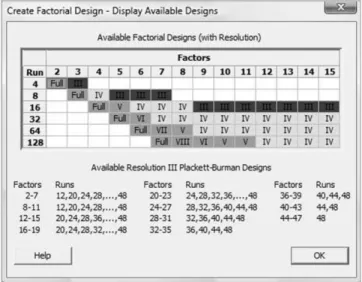
Use was then made ofStat>DOE>Factorial>Create Factorial Design. . .with the option2-level factorial (default generators)selected underType of Design. Part of the dialog is shown in Figure 8.19.Number of factors: was specified as 2. UnderDesigns . . . the only available design is the full factorial design. The number of FLCs is 22¼4, so Minitab indicates this by listing the number ofRunsrequired as 4.Resolution, Full in this case, will be discussed later in the chapter. Minitab represents 22as 22. TheNumber of replicates:was specified as 2, theNumber of blocks:as 1 andNumber of center points:as 0. (Experimental designs involving centre points will be considered in Chapter 10.)
Observed data value¼Overall meanþBottle effectþOperator effect þRandom error
Yijk ¼mþaiþbjþeijk; i¼1;2;. . .;a; j¼1;2;. . .;b; k¼1;2;. . .;n aiNð0;s2aÞ; bjNð0;s2bÞ; eijkNð0;s2Þ
(The random variablesai,bjandeijkare independent.)
Box 8.4 Revised random effects model.
Expected Mean Square for Each Term (using Variance Error unrestricted Source component term model)
1 Bottle 0.00934 3 (3) + 6 (1)
2 Operator 0.00009 3 (3) + 20 (2)
3 Error 0.00023 (3)
Panel 8.8 Estimated variance components from revised model.
On clickingOKone may commence the remainder of the dialog. UnderFactors. . .the factors temperature and pressure (both numeric in this case) and their levels were specified.
The defaults were accepted underOptions. . ., i.e. toRandomize runsand toStore design in worksheet. (No reference will be made in this book toFold DesignandFraction.) Under Results. . .the defaults were also accepted. On clickingOK,OKthe resulting worksheet should be augmented with a column in which the values of yield obtained can be recorded and a column in which those carrying out the experiment can note any unusual happening or information that might prove relevant to the analysis of the data from the experiment and to the project. Before commencing the experimentation the work to date should be stored in a Minitab project. Fictitious yield data are used in order to make the checking of key calculations straightforward for the reader.
Once the experiment has been completed one could carry out the display and analysis using facilities for plotting and analysis available underStat>ANOVA>. . ., but Minitab has built- in facilities for the analysis of 2kfactorial experiments viaStat>DOE>. . .. For initial display of the data one may useStat>DOE>Factorial>Factorial Plots. . .. The data and dialog involved in the creation of the three plots available are shown in Figure 8.20. The data are provided in Reactor1.MTW and the reader should use that worksheet should he/she wish to re-create the displays and analysis that follows as the worksheet, which was created using Stat>DOE>Factorial>Create Factorial Design. . ., includes hidden stored information on the experimental design.
Main Effects Plot,Interaction PlotandCube Plotwere all checked. Once a plot type has been checked one must then click on the corresponding Setup. . . button and enter the Responsesto be plotted andFactors to Include in Plots. The arrow keys may be used to select or deselect highlighted factors from the list of Available: factors. Both temperature and pressure were selected for all three plots, the defaults. For all three plots the default option to display Data Meansas Type of Means to Use in Plotswas accepted. In the case of the interaction plot the option toDraw full interaction plot matrixwas selected in order to obtain the display in Figure 8.22. (The reader should note that specification of a response is optional in the case of the cube plot. This allows experimenters, who wish to do so, to create a blank cube plot on which they can record data means for discussion prior to any formal analysis using software.)
The left-hand component of the annotated main effects plot in Figure 8.21 has the mouse pointer located at the point representing the mean yield of 88 kg from all the experimental runs
Figure 8.19 Dialog for design of a 22experiment.
FULL FACTORIAL EXPERIMENTS IN THE 2kSERIES 327
carried out with temperature 200C, as can readily be verified from the data in the worksheet in Figure 8.20. The mean yield from all the experimental runs carried out with temperature 250C was 96 kg. Hence, on average, increasing temperature from 200C to 250C increases yield of product by 8 kg. The reader is invited to confirm that the right-hand component of the plot indicates that, on average, increasing pressure from 4 bar to 5 bar decreases yield of product by 6 kg. The main effect of temperature is 8 kg and the main effect of pressure is 6 kg.
Both versions of the interaction plot are shown in Figure 8.22. The mouse pointer is placed over the point in one version that corresponds to the FLC with temperature 250C and pressure
Figure 8.21 Main effects plot for reactor 1.
Figure 8.20 Dialog for creating factorial plots.
5 bar. Scrutiny of the data table visible in the worksheet in Figure 8.20 reveals yields of 90 and 96 kg with mean 93 kg. The parallel lines indicate no temperature–pressure interaction in this situation. The reader is encouraged to create the plot in Figure 8.22 for him/herself and, with a copy of the data at hand, to move the mouse pointer to each of the eight points in turn and confirm the mean yields displayed.
The mean yields for the four FLCs used in the experiment are plotted at the vertices of a square (a cube in two dimensions!) in the cube plot in Figure 8.23. The annotated version of the cube plot in Figure 8.24 indicates another way of determining the main effect of temperature. The annotated version of the cube plot in Figure 8.25 indicates another way of determining the main effect of pressure.
Figure 8.22 Interaction plots for reactor 1.
Figure 8.23 Cube plot for reactor 1.
FULL FACTORIAL EXPERIMENTS IN THE 2kSERIES 329
Having displayed the data in various ways, the next step is to perform the formal analysis usingStat>DOE>Factorial>Analyze Factorial Design. . .. (Note that the Minitab icon forAnalyze Factorial Design. . .is based on the sort of cube plot we have been considering in Figure 8.23.) The dialog is shown in Figure 8.26.
It is necessary to specify Yield underResponse:and to specify the model usingTerms. . ..
Here underTerms:A: Temperature, B: Pressure and AB, denoting the temperature–pressure interaction, are selected as the default. Part of the Session window output obtained is shown in Panel 8.9.
Figure 8.24 Annotated cube plot for main effect of temperature.
Figure 8.25 Annotated cube plot for main effect of pressure.
Note that the temperature effect of 8 and the pressure effect of –6 estimated from the data earlier are given in the first column. The interaction plots indicated no temperature–pressure interaction and this corresponds to the interaction effect estimate of zero. (The redundant negative sign will have arisen due to the way that numbers are stored in the software.) The Coef (coefficient) column in the output has the value 92 as the first entry. This is the overall mean yield for the entire experiment and is referred to as the constant term in the model. The coefficients corresponding to temperature, pressure and temperaturepressure are simply half the corresponding effects. (Equations in which these coefficients are required will be discussed later in the chapter.) The heading SE Coef refers to the standard errors of the coefficients. For example, the constant term 92 is the mean of a sample of eight measurements.
The standard error or standard deviation of a mean of eight values is the standard deviation for individual values divided by ffiffiffi
p8
. The output gives the estimated standard deviation of individual yields obtained from the ANOVA to be s¼2.645 75. Division by ffiffiffi
p8
yields 0.9354. The values of the coefficients divided by their standard errors give a Student’s t-statistic for testing the null hypothesis that each coefficient is zero. TheP-values for each are given in the final column. The fact that theP-values for both temperature and pressure are less than 0.05 may be taken as evidence that both temperature and pressure have a real effect on
Figure 8.26 Analysing the factorial experiment.
Estimated Effects and Coefficients for Yield (coded units) Term Effect Coef SE Coef T P Constant 92.000 0.9354 98.35 0.000 Temperature 8.000 4.000 0.9354 4.28 0.013 Pressure -6.000 -3.000 0.9354 -3.21 0.033 Temperature*Pressure -0.000 -0.000 0.9354 -0.00 1.000
S = 2.64575 PRESS = 112
R-Sq = 87.72% R-Sq(pred) = 50.88% R-Sq(adj) = 78.51%
Panel 8.9 ANOVA for 22factorial experiment on reactor 1.
FULL FACTORIAL EXPERIMENTS IN THE 2kSERIES 331
yield. However, as suspected from viewing the interaction plots, there is no evidence of a nonzero temperature–pressure effect.
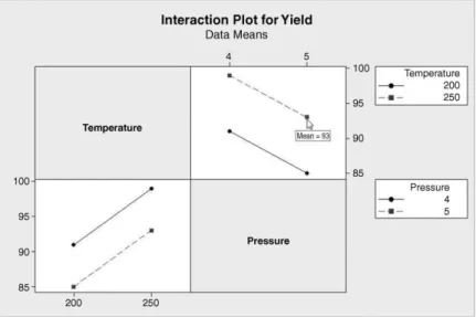
Consider now an experiment, with the same design as above, performed on reactor 2, a different type from reactor 1. Currently, as with reactor 1, the process is also operated at temperature 225C and pressure 4.5 bar, and yields average 90 kg. The data are available in Reator2.MTW, and the reader is invited to create a cube plot for this second experiment and to verify that the main effects for temperature and pressure are 8 and 6, respectively. One version of the interaction plot for reactor 2 is displayed, with annotation, in Figure 8.27. The nonparallelism suggests the presence of a temperature–pressure inter- action effect.
. When pressure was set at 5 bar the effect of increasing temperature from 200 to 250C was to increase mean yield, on average, from 87 to 91 kg, i.e. by 4 kg.
. When pressure was set at 4 bar the effect of increasing temperature from 200 to 250C was to increase mean yield, on average, from 89 to 101 kg, i.e. by 12 kg.
. The main effect of temperature is given by (4þ12)/2¼8.
. The temperature–pressure interaction effect is given by (4 12)/2¼ 4.
In the final calculation of the interaction effect it is important to note that the difference considered is that of the effect of temperature at the higher level of pressure less that of the effect at the lower level of pressure. (Had the changes in mean yield, indicated by the arrows in Figure 8.27, been equal then the line segments linking points with the same level of temperature in the interaction plot would have been parallel, as in the top right- hand panel in Figure 8.22. The difference between the changes would be zero and the interaction effect would be zero.) The second version of the interaction plot is shown in Figure 8.28.
Figure 8.27 First version of interaction plot for reactor 2.
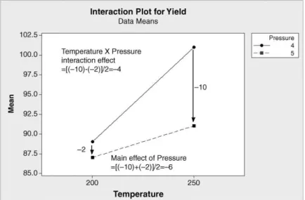
. When temperature was set at 250C the effect of increasing pressure from 4 to 5 bar was to change mean yield, on average, from 101 to 91 kg, i.e. by 10kg.
. When temperature was set at 200C the effect of increasing pressure from 4 to 5 bar was to change mean yield, on average, from 89 to 87 kg, i.e. by 2 kg.
. The main effect of pressure is given by [( 10)þ( 2)]/2¼ 6.
. The temperature-pressure interaction effect is given by [( 10) ( 2)]/2¼ 4.
The reader is also invited to verify using Stat>DOE>Factorial>Analyze Factorial Design. . .that the output in Panel 8.10 is obtained. Note that the effects calculated earlier are confirmed and also that the interaction effect differs significantly from zero at the 10% level of significance. Thus there is slight evidence of a real temperature–pressure interaction in the case of reactor 2.
Montgomery (2009, p. 566) gives an example from the electronics industry. It concerned registration notches cut in printed circuit boards using a router. Although the process was stable, producing a satisfactory mean notch size, variability was too high. High variability leads to problems in assembly, when components are being placed on the boards, due to
Figure 8.28 Second version of interaction plot for reactor 2.
Factorial Fit: Yield versus Temperature, Pressure
Estimated Effects and Coefficients for Yield (coded units) Term Effect Coef SE Coef T P Constant 92.000 0.7906 116.37 0.000 Temperature 8.000 4.000 0.7906 5.06 0.007 Pressure -6.000 -3.000 0.7906 -3.79 0.019 Temperature*Pressure -4.000 -2.000 0.7906 -2.53 0.065
Panel 8.10 ANOVA for 22factorial experiment on reactor 2.
FULL FACTORIAL EXPERIMENTS IN THE 2kSERIES 333
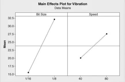
improper registration. The engineers associated with the process reckoned that the high variability was due to vibration and decided to use a 22factorial experiment, with four replications, to investigate the effect of the factors bit size and speed on the response vibration, as measured using accelerometers attached to the boards. The reason for choosing vibration as the response was that variability in notch dimension was difficult to measure directly but it was known that vibration correlated positively with variability. The levels were 1/16 inch and 1/8 inch for bit size, and 40 rpm and 80 rpm for speed. Vibration was measured in cycles per second. The design and the data, reproduced by permission of John Wiley & Sons, Inc., New York, are stored in Vibration.MTW.
Use ofStat>DOE>Factorial>Analyze Factorial Design. . . yields the output in Panel 8.11. AllP-values are less than 0.001, which indicates, in particular, that we have strong evidence of interaction between bit size and speed.
The main effects plot is shown in Figure 8.29. Na€ıve scrutiny of the main effects plot would suggest that the combination of small bit size with low speed would be best in terms of keeping vibration as low as possible. However, running the process using low speed would have had major implications in terms of process throughput. The major interaction between bit size and speed provided a resolution to this issue. The interaction plots are presented in Figure 8.30. These plots reveal that, with bit size 1/16 inch, vibration is low at both speeds 40 rpm and 80 rpm. Thus it was decided to operate the process with bit size 1/16 inch and speed 80 rpm. This led to a major reduction in the variability of the size of the registration notches.
The residual plots are shown in Figure 8.31. They were created usingGraphs. . . in Analyze Factorial Design. . .with theFour in oneoption selected. Although the variability of the set of residuals for the lowest of the four fitted values appears relatively low, use of Stat>ANOVA>Test for Equal Variances. . .withResponse:Vibration andFactors:Bit Size Speed yields no formal evidence of nonconstant variability. The plots appear to be generally satisfactory.
8.2.2 Models and associated displays
In order to introduce further important ideas some notation is required. Were one to design a 22 experiment with no centre points, one replication, no blocking, no randomization of the run order and using the factor names X1 and X2, with the default levels, then the worksheet displayed in Figure 8.32 would be obtained. The columns named X1 and X2 in the worksheet contain the essence of the design. The X1X2 interaction effect may be calculated by using an additional column X1X2. This additional X1X2 column may be obtained from the X1 and X2 columns by simply multiplying corresponding row entries together, hence the X1X2 notation.
Factorial Fit: Vibration versus Bit Size, Speed
Estimated Effects and Coefficients for Vibration (coded units) Term Effect Coef SE Coef T P
Constant 23.831 0.6112 38.99 0.000 Bit Size 16.638 8.319 0.6112 13.61 0.000 Speed 7.538 3.769 0.6112 6.17 0.000 Bit Size*Speed 8.713 4.356 0.6112 7.13 0.000
Panel 8.11 ANOVA for 22factorial router experiment.
In terms of the reactors referred to earlier, X1 and X2 may be considered as coded variables representing temperature and pressure, respectively. Recall that current operating conditions were temperature 225C and pressure 4.5 bar. These would have coded values X1¼0 and X2¼0, respectively. The high level of temperature used in the experiment, i.e. 250C, would be coded as X1¼1 and the low level, 200C, as 1. Similarly, the low and high levels of pressure used, 4 bar and 5 bar, would be coded as X2¼ 1 and X2¼1, respectively.
The author finds it helpful to think in terms of a reactor control panel as shown in Figure 8.33. The low temperature of 200C is ‘one notch down’ (X1¼ 1) from the current
Figure 8.29 Main effects plot for router experiment.
Figure 8.30 Interaction plots for router experiment.
FULL FACTORIAL EXPERIMENTS IN THE 2kSERIES 335
Figure 8.31 Residual plots for router experiment.
Figure 8.32 Basic 22design in standard order.
Figure 8.33 Reactor control panel.
operational setting and the high pressure of 5 bar is ‘one notch up’ (X2¼1) from the current operational setting.
Table 8.10 lists the four FLCs used in the experiment with reactor 1. The means in the final column are the means of the pairs of yields obtained with each FLC. The overall mean and effects may be calculated as follows. The overall mean is simply (91þ99þ85þ93)/
4¼92. The main effect of temperature is given by Mean yield with X1¼1
½ ½Mean yield with X1¼ 1
¼99þ93 2
91þ85
2 ¼96 88¼8:
The main effect of pressure is
Mean yield with X1¼1
½ ½Mean yield with X2¼ 1
¼85þ93 2
91þ99
2 ¼89 95¼ 6:
Finally the temperature–pressure interaction effect is given by Mean yield with X1X2¼1
½ ½Mean yield with X1X2¼ 1
¼91þ93 2
99þ85
2 ¼92 92¼0:
These calculations are summarized in Table 8.11. Each coefficient is half the correspond- ing effect.
Table 8.12 lists the four FLCs used in the experiment with reactor 2. The means in the final column are the means of the pairs of yields obtained with each FLC. The reader is invited to check the calculation of the three effects and corresponding coefficients displayed in Table 8.13 and to confirm that the overall mean is 92.
Table 8.10 Reactor 1 data.
FLC X1 X2 X1X2 Mean Y
1 1 1 1 91
2 1 1 1 99
3 1 1 1 85
4 1 1 1 93
Table 8.11 Reactor 1 effects.
Mean response at level þ
Effect Coefficient
X1 88 96 8 4
X2 95 89 –6 –3
X1X2 92 92 0 0
FULL FACTORIAL EXPERIMENTS IN THE 2kSERIES 337
The constant (overall mean) and the coefficients generated by Minitab provide statistical models for the expected response of the form
Y¼Overall meanþCoeff:of X1X1þCoeff:of X2X2 þCoefficient of X1X2X1X2:
For reactor1 we obtain
Y¼92þ4X1 3X2þ0X1X2¼92þ4X1 3X2;
and for reactor 2 we have
Y¼92þ4X1 3X2 2X1X2
The models are of the formY¼f(X) referred to in Section 1.4. Here the bold X represents the pair of factors X1 and X2. The model may be used to predict the expected yield for any FLC.
(The models may also be obtained using multiple regression methods that will be referred to in Chapter 10.) As an example, consider reactor 1 operating at temperature 250C (X1¼1) and pressure 4 bar (X2¼–1). Substitution of these values into the reactor 1 model equation gives expected yield
Y¼92þ41 3 ð 1Þ ¼92þ4þ3¼99:
Of course this is the mean yield obtained for reactor 1 with temperature 250C and pressure 4 bar in the experiment and is the fitted value from the model for the particular FLC of temperature 250C and pressure 4 bar.
As a second example, consider reactor 2 operating at temperature 200C (X1¼–1) and pressure 5 bar (X2¼1). Substitution of these values into the reactor 2 model equation gives expected yield
Y¼92þ4 ð 1Þ 31 2 ð 1Þ 1¼92 4 3þ2¼87:
Table 8.12 Reactor 2 data.
Reactor 2 Coded Factor Levels
FLC X1 X2
X1X2 Mean Y
1 1 1 1 89
2 1 1 1 101
3 1 1 1 87
4 1 1 1 91
Table 8.13 Reactor 2 effects.
Mean response at level þ
Effect Coefficient
X1 88 96 8 4
X2 95 89 6 3
X1X2 94 90 4 2
This is the mean yield obtained for reactor 2 with temperature 200C and pressure 5 bar in the experiment and is the fitted value from the model for that particular FLC.
In terms of optimizing the performance of the reactors by achieving as great a yield as possible, it would appear that both operate best, in the ranges of temperature and pressure considered in the experiments, at temperature 250C and pressure 4 bar. The ranges of factor levels considered in an experiment constitute the design space. With the reactor models above it is a fairly simple matter to substitute coded values of temperature and pressure into the model equations to obtain predicted responses.
Minitab provides a facility for investigation of process optimization using the models fitted to data from 2kfactorial experiments. With worksheet Reactor2.MTW open, for example, this facility is available viaStat>DOE>Factorial>Response Optimizer. . .. Recall that the reactors have been achieving yields averaging 90 kg with the current operating settings of 225C and 4.5 bar. Suppose that the project team had decided that it was desirable to achieve yields as high as possible, with target 105 kg on average and no worse than 95 kg on average.
The Response Optimizer may be used to explore model predictions in a visual way and without having to perform calculations directly from the model equations. Part of the necessary dialog is shown in Figure 8.34.
It is necessary here to haveSelected:Yield as the (only) response and underSetup. . .to set Goalto Maximize,Lowerto 95 andTargetto 105. No value is entered forUpperwhen seeking to maximize a response.WeightandImportanceneed not concern us when dealing with a single response. UnderOptions. . .check onlyOptimization Plot; there is no need to enter anyStarting valuefor the factors.
The outcome from implementation is an interactive screen, part of which has been captured in Figure 8.35. The reader is advised to have this screen on display on his/her computer for the
Figure 8.34 Dialog for Response Optimizer.
FULL FACTORIAL EXPERIMENTS IN THE 2kSERIES 339