Our effective price stabilization index measures the proportion of inflationary pressures that were dampened by the policies implemented by the monetary authority. According to (3), there is a trade-off between inflation and the interest rate, for givenxet,et, andut. An index value of 0 indicates that the monetary authority did not succeed in alleviating some of the underlying inflationary pressures.
Index values between 0 and 1 reflect the proportion of inflation stabilization achieved by the monetary authority's policy initiative. 5 The concept of ex post inflationary pressure is analogous to the concept of exchange market pressure introduced by Weymark. An index value of 0 means that the policy was effective in removing all inflationary pressures from the economy.
However, when P Et = 1, monetary policy is ineffective in reducing the level of inflationary pressure. When ex ante inflationary pressure is positive, an index value greater than 1 means that monetary policy has increased inflationary pressure.
Illustration of the Methodology
The first step in deriving measurements consistent with the ex ante inflation pressure model and the monetary policy response is to obtain the rational expectations solution for our model. When the actual value of ρ is less than unity (i.e., 0 ≤ρ < 1), the ex ante inflationary pressure measures, therefore, a full predicted one-period deviation from the observed interest rate rule ( mean) given in (9). Ex post inflationary pressure is the inflationary pressure that remains after the monetary policy response has taken effect.
In Figure 1, ex post inflation pressure in periodt is given as the vertical distance between the two feasibility constraints, IR0 and IR1, at dit-1. However, we can use our theoretical model to derive an operational formula for ex post inflationary pressure that can be calculated based on observed changes in inflation and interest rate levels. In the context of our model, ex post inflationary pressure in period t is measured as the change in inflation that would be generated by ut, et, and it−1, given the expectations formulated under the policy actually implemented (i.e. under .
The Quarterly Model
Therefore, our measure of inflationary pressure captures the effect on inflation of a very specific one-period deviation from the interest rate rule. The variables Xtη and Xtε consist of weighted sums of current and/or lagged changes in the interest rate, the inflation rate and the output level. 8Note that because (25)-(28) include lagged variables, our quarterly measure of ex ante inflation pressure for a given period captures not only the impact of current exogenous disturbances but also the impact of past policy actions that reflected in values of lagged endogenous variables.
In the context of a quarterly empirical model, our ex ante index of inflation pressure measures the inflation rate that would have been observed in periodt, taking policy in periodt−4 and earlier as given, if there had been no change in the interest rate between periods took place. −3 ent−2. However, to the extent that past policy actions contribute to the inflationary environment facing the policy authority in a given period, our ex ante inflation pressure index still provides a useful benchmark against which to measure the strength and effectiveness of the monetary authority's policy response. Ex post-inflationary pressures, πtw − πt−1, measures the inflationary pressures remaining after the implementation of monetary policy (measured as interest rate changes).
Given the two-period control lag in our model, ex post inflationary pressure in period t is measured in terms of the observed change in inflation in period t and the observed change in the interest rate from period t−3 to period t−2 . The formula for ex post inflationary pressure corresponding to our quarterly model is To calculate our inflation pressure indices, we need estimates of the coefficients in our model as well as the rational expectations solutions for the endogenous variables πt, yt, and it.
Details of the numerical methods used to obtain the rational expectations solutions for these variables are given in Appendix 2. Two types of expectation variables appear in our model, they reflect the expectations that private actors form about future inflation and the future output gap . Rudebusch (2002) uses, for example, The Michigan Survey of Inflation Expectations to estimate a quarterly version of (8) by OLS.
Inflation is defined as ≡100 (lnPt−lnPt−1) where Pt is the price index weighted by the GDP chain.
Estimated Indices for the United States
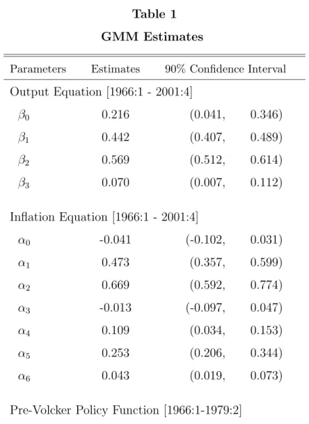
The signs of all our unconstrained parameter estimates are consistent with theory and also with the results obtained in previous studies. Note, however, that Clarida, Gal´ı, and Gertler (2002) found that γπ was below unity for the pre-Volcker period and greater than unity thereafter. The results in Table 1 show that the γπ estimates are greater than unity for both the Pre-Volcker and Volcker-Greenspan periods.
This is consistent with Inoue and Shintani (2004), who find that the hypothesis that γπ exceeds unity cannot be rejected for the pre-Volcker period. The results obtained using the HP filtered data are quite similar to those obtained using the CBO output gap, so they are not reported here. Fuhrer and Rudebusch (2002) showed that GMM estimators can exhibit finite sample bias, making asymptotic standard errors unreliable indicators of statistical significance.
We addressed this problem by using Inoue and Shintani's (2003) block bootstrapping procedure, which is designed to improve the finite sample standard error properties of GMM estimators with correlated errors.
A Quantitative Characterization of Federal Reserve Policy
This means that inflation would have fallen about fifty percent of the time even if the Fed had made no interest rate changes. The PE value of 0.57 indicates that the monetary policy implemented by the Fed led to a 43 percent decline. in inflation expectations. According to our index, ex ante inflationary pressures were negative in the two quarters prior to the September 2001 terrorist attack.
For each sub-period, we calculated average values for the output gap, changes in observed inflation and previous inflation pressure (IP). The last two columns of Table 5 show average measures of the impact of Fed policy on inflation expectations (PE). The data show that the average inflation rate was positive during the first three years of Greenspan's tenure, then negative thereafter.
However, our EPS indices show that monetary policy under Martin and Burns was also effective in reducing inflationary pressures. Monetary policy under Martin and Burns removed an average of 27 and 19 percent of positive ex ante inflationary pressure, respectively. The PE index measures the degree to which changes in expectations have contributed to the Fed's success in combating inflationary pressures.
According to our estimates, monetary policy increased the level and volatility of inflation on average. However, our inflation pressure indices show that the decline in inflation during this period was due not only to the effectiveness of Fed policies, but also to exogenous deflationary forces. The reward for this commitment is also clearly visible in the PE index, which shows that the Fed's policies lowered inflation expectations by 36 percent.
By implementing somewhat stronger contractionary policies when inflationary pressures were positive and continuing to contract strongly in deflationary quarters, the Fed increased the mag-. In the last 5 years of our sample, the output gap was moderately positive and, due to productivity growth, inflationary pressure was negative. Greenspan's response to negative and positive inflation pressure was less aggressive than in previous years.
Concluding Comments
Nevertheless, these policies served to increase ex ante deflationary pressure by 50 percent, bringing inflation (as measured by the GDP deflator) down to 2.13 percent by the end of 2001.
A New Test in the Spirit of Friedman and Schwartz,” in Olivier Blanchard and Stanley Fischer (eds), NBER Macroeconomic Annual (Cambridge MA: MIT Press). 2002) “Assessing Nominal Income Rules for Monetary Policy with Model and Data Uncertainty,” Economic Journal. The perturbation terms ηt−1, εt−1 andεt in (A.12) are unobservable and must be obtained by solving (A.3) and (A.4) simultaneously for ηt and εt. In the quarterly model, ex ante inflationary pressure is measured as the inflation rate that would have been observed if the monetary authority had kept interest rates constant at the level of period t−3 in period t−2 and then returned to the average policy rule. for subsequent periods.
Since economic agents are assumed to be fully informed and fully rational, the coefficients in (A.3)-(A.5) that would be obtained under the counterfactual assumption ρt−2 = 1 can be expected to differ from those obtained under the policy . rule that was actually implemented. Unfortunately, the complexity of the quarterly model prevents us from obtaining closed-form solutions for the coefficients that would be generated by a one-period deviation from the policy rule. Therefore, we approach the solution by forming expectations using the coefficients calculated according to the observed rule.
This approximation is unlikely to have any significant effect on the Volcker-Greenspan estimates because the estimated value of ˆρ = 0.8 is very close to 1. However, even in this case there should be little effect since we only omit to adjust the coefficients for a one-period deviation from the estimated policy rule. The defining equations associated with these vectors and to be added to the system are.
The solutions for the undetermined coefficients in (A.3)–(A.4) were obtained by using the GMM estimates for the coefficients in (25)–(28) to perform the calculation described above. We therefore used the heteroscedasticity and autocorrelation consistent (HAC) procedure using a Bartlett kernel with bandwidth K = 4 (or lag length 3) to calculate the optimal weighting matrix in the GMM criterion and also to calculate the standard errors.
