The presence of these nonadiabatic couplings (even if they are not singular) can lead to numerical inefficiencies in solving the corresponding nuclear motion Schr¨odinger equation. An important consequence of the presence of degenerate electronic states is the geometric phase effect.
Introduction
Due to the small ratio of the electron mass to the total mass of the nuclei, ν ≈ mel. The electronic Hamiltonian and the corresponding eigenfunctions and eigenvalues are independent of the orientation of the nuclear-body fixed frame with respect to the space-fixed one and thus depend only on qλ.
Born-Huang expansion
Adiabatic nuclear motion Schr¨odinger equation
The Schrödinger equation of the nuclear motion in n-electronic state satisfied by χad(Rλ) can be obtained by inserting Eqs. All matrices appearing in this n-electronic state nuclear motion Schrödinger equation [Eq. 2.15)] are-dimensional diagonal except W(1)ad and W(2)ad, which are the first and second derivative [1, 7–13] nonadiabatic coupling matrices, respectively, discussed below.
First-derivative coupling matrix
These coupling matrices allow nuclei to sample more than one adiabatic electronic state during a chemical reaction and thus change its dynamics in an electronically non-adiabatic manner. If the Cartesian components of Rλin 3(Nnu−1) of the nuclear configuration space fixed in space are Xλ1, Xλ2, .., Xλ3(Nnu−1), the corresponding Cartesian components of wi,j(1)ad(Rλ) are. 2.10) and therefore its diagonal elements w(1)adi,i (Rλ) are pure imaginary quantities.
Second-derivative coupling matrix
In addition, the presence of the first-derivative gradient term W(1)ad(Rλ) ·∇R. 2.15), even for a nonsingular W(1)ad(Rλ) (e.g., for avoided crossings), introduces numerical inefficiency in solving that equation. Because they are scalars, the second-derivative couplings can be easily included in the scattering calculations without any additional computational effort.
Adiabatic-to-diabatic transformation
Electronically diabatic representation
If the electronic wave functions in the adiabatic and diabatic representations are chosen to be real, as is usually the case, U(qλ) is orthogonal and therefore has n(n −1)/2 independent elements (or degrees of freedom). This transformation matrix U(qλ) can be chosen to provide a diabatic electronic basis set with desired properties, which can then be used to derive the diabatic nuclear motion Schr¨odinger equation. 2.27) and (2.28) and the orthonormality of the diabatic and adiabatic electronic basis sets, we can relate the adiabatic and diabatic nuclear wave functions through the same.
Diabatic nuclear motion Schr¨odinger equation
The presence of this term can also introduce problems of numerical inefficiency in solving Eq. Since the ADT matrix U(qλ) is arbitrary, it can be chosen to make Eq. 2.31) have desirable properties that Eq.
Diabatization matrix
In the adiabatic representation, the GP effect must still be imposed on each of the two state nuclear wave functions. The equilateral triangle (C3v) configuration of H3 corresponds to a conical intersection between the ground and the first excited electronic states of the system.
Theory and numerical methods
Ab initio couplings and electronic energies
A three-dimensional cubic interpolation [69] of the first derivative coupling vector components is performed using all 784 geometries. This angle is the integral of the closed path of the cross section of the coupling of the first outlet.
DMBE couplings and electronic energies
The original DMBE code was used in this work to obtain these longitudinal couplings and the two lowest PESs for H3. 3.3 the two lowest DMBE PESs of H3 are compared with the PESs obtained from the fits of the ab initio energies.
Ab initio and DMBE electronic energies
Fitting method
This procedure is performed for both the ground PESs and the first-excited PESs, and the resulting PESs are examined with the help of equipotential contour plots in the corresponding Cartesian space with two internuclear distances at fixed bond angles for each feature of false in these PES. These fitted DSP PESs are also examined in hyperspherical coordinates with the help of equipotential contour plots at fixed hyperbeams, as discussed in the next subsection, and compared to the corresponding contour plots for DMBE PESs.
DSP and DMBE potential energy surfaces
The corresponding xλ and yλ of the Q-map of the point P in the tangent plane are then. 3.1 (a) to (d) show the equatorial views of the equipotential contours of the 1 2A0 surface for the DSP (E1DSP) fit to the ab initio data at constant values of the hyperradiusρ.
Results and discussion
Ab initio and DMBE first-derivative couplings
The Cartesian components of the longitudinal part of the DMBE first-derivative coupling vector are also obtained from Eq. The second in units of bohr−1 corresponds to the three-dimensional space sampled by the x, y, and z components of the coupling vector.
The topological phase
Discussion
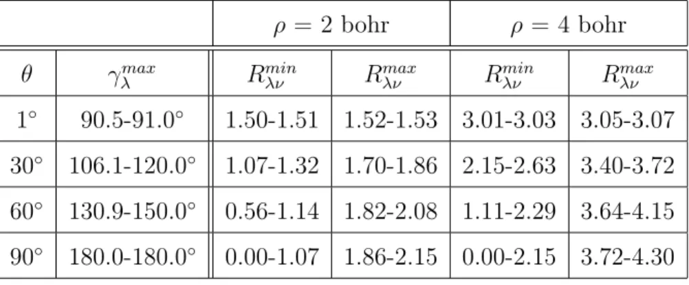
A similar detailed analysis of the coupling vectors of the first derivative of DMBE (Figures 3.8 to 3.11) leads to the following conclusions. For ρ = 2 bohr (Figure 3.8), the coupling vector has a z-component that is negligible near the conical intersection (θ = 1◦) and at collinear geometries (θ = 90◦), but non-negligible in the intermediate regions. It shows the singular behavior of diagonal elements W(2)ad(qλ) for conical intersection geometries (θ = 0◦).
Elements of the diabatic matrix W(2)d are usually small near a conical intercept and can be added to εd to obtain a corrected diabatic matrix. As a result, the longitudinal and transverse parts of the first derivative torque vector are referred to.
Methodology
- Coordinate system
- The Poisson equation
- Boundary conditions for solving the Poisson equation
- Numerical solution of the Poisson equation
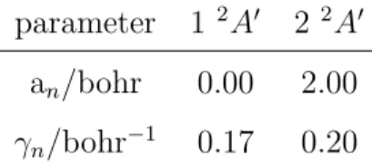
An approximate analytical expression for β(ρ, θ, φλ) was obtained by Varandas et al [47] using the double multipart expansion (DMBE) of the two lowest. In the DMBE treatment, the transverse part of the coupling vector of the first lead is assumed to be negligible (especially near the conical intersection) compared to the longitudinal part. This angle was then used in Eq. 4.29) to obtain the cross section of the coupling vector of the first derivative.
Results and discussion
Diabatization angle
In the next section, we present the results obtained for the diabaticization angle as well as those for the longitudinal and transverse parts of the first-derivative coupling vector. This negligibly small magnitude of the coupling vector leads to its negligible divergence as indicated by the source termσ(ρ, θ,3φλ) shown in panels (c), (d), (g) and (h) of Figs. 4.7, ∆ γ is plotted as a function of θ for the same four values of the hyperradius ρ, as this provides an indication of the ρ-dependent difference between γDMBE and γ as a function of θ.
Longitudinal and transverse parts of the first-derivative cou-
The cases θ = 30◦ and θ = 60◦ (panels (b) and (c), respectively) are included to evaluate the importance of the coupling vector away from the conical intersection as well as from collinear geometries. We can now check whether they(1)adlon andwtra (1) described above satisfy Eq. 4.27), which are consequences of the geometric phase theorem. The corresponding topological phase values ΦT,lon(ρ, θ) and ΦT,tra(ρ, θ) can be read from these panels by taking the phases of the open path at φλ = 2π (or 360◦).
Diabatic potential energy surfaces
In the next section, we will discuss the characteristics of the adiabatic and diabatic PESs according to their contours shown in Fig.
Discussion
This analysis shows that even the transverse part of the ab initio is first derivative. This should manifest itself by the z-component of the transverse vector being zero (due to Eq. A comparison of the transverse coupling vectors (Fig. 4.10) with their longitudinal counterparts (Fig. 4.9) leads to the following conclusions.
A similar comparison of the rightmost column (ρ = 8 bohr) shows that its magnitude is 10 to 50 times larger than that of the optimal wtra(1)ad vector. The lower side of the panels is similar to those of the corresponding panels of Fig.
Symmetrized hyperspherical coordinates
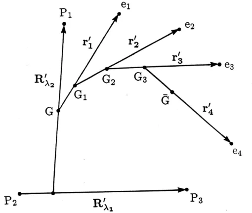
Let GxIλyIzIλ be a body-fixed frame Iλ, whose axes are the main axes of inertia of the three cores and whose Euler angles with respect to the space-fixed frame Gxsfysfzsf are aλ, bλ, cλ with G the center of mass of the three cores. Jˆ±Iλ= ˆJxIλ±iJˆyIλ (5.15) JˆxIλ, ˆJyIλ and ˆJzIλ are the components of the total orbital angular momentum ˆJ of the nuclei in the Iλ frame. The angular momenta associated with these operators are related to the total orbital angular momentum ˆJ of the nuclei.
Adiabatic formalism
Partial wave expansion
As a result, Ψo(r,Rλ) appearing in Eq. 5.21) must be transformed according to an irreducible representation Γ of the corresponding permutation group. We will use this boundary condition to choose appropriate basis functions, in the absence or presence of the conical intersection, for the expansion of the nuclear wave functions as discussed next. Using the orthonormality of the symmetric Wigner functions [Eq. 5.41)] and integration over the two-dimensional adiabatic LHSFs on the hypergons θ, φλ for the strong interaction region gives a set of second-order hyperradial ordinary differential equations (also called coupled channel equations) in the coefficients sin, JΠΓn1 ,n1 0λΩ0λ.
Propagation scheme and asymptotic analysis
Vad,JΠΓ(ρ; ¯ρ) is the interaction potential matrix obtained from this derivation procedure and which includes ad(¯ρ) and the matrices with parts defined in Eq. At the transition hyperradius (ρs) separating the strong and weak interaction regions, the overlap matrix is calculated by first projecting the two-dimensional LHSFs (θ, φλ) in the last sector of the strong interaction region into the space ωλ, γλ and then computing its overlap with the two-dimensional LHSFs (θ, φλ) in the first sector of the weak interaction region. For the total energies at which the electronically excited states of isolated atoms or diatomic molecules are not open, the elements of the open parts of these matrices correspond only to the ground electron atom and diatom products.
Diabatic formalism
Partial wave expansion
As we did in the adiabatic case, we can write the diabatic nuclear motion of the Schr¨odinger equation. As in the case of the adiabatic treatment, the singularities in the ˆΛ21operator of Eq. Furthermore, in the current diabatic case, the second-derivative coupling element added to the diabatic energies [see Eq.
Propagation scheme and asymptotic analysis
Adiabatic vs. diabatic approaches
In the adiabatic representation of a system containing singular couplings at the conical intersection geometries, second-derivative couplings have a second-order pole compared to first-derivative couplings. In energy units, this translates to nuclear wavefunctions that do not sample the conical intersection geometries or their very close vicinity, where the second-derivative coupling can still be large. These second-derivative couplings decay faster than the first-derivative ones as we move away from the conical intersection, and the presence of the first-derivative couplings in the gradient term mentioned above will still render the solution of the adiabatic equations inefficient.