First of all, I would like to thank my advisor Larry Rolen for his guidance and support during my graduate studies, without which this thesis would not have been possible. I am also very grateful to my family who have been incredibly supportive throughout my graduate program.
Partitions
In addition, it appears that the derivative of sinh appearing in (I.1) can be rewritten as an I-Bessel function, which we will define by. We will use this exact formula in Section IV to prove inequalities for fractional partitions.
Note that all 4 cores are of one of the shapes above by simply ordering the number of beads in each column. The number of rows of the corresponding Frobenius partition is given by the main diagonal, which in this case is three.
Ramanujan’s congruences and beyond
The values ofk (mod`) classifying the existence of congruences in theorems I.3.1 and I.3.3 may seem arbitrary at first glance. As a result, we must regard Theorems I.3.1 and I.3.3 only as partial progress toward classifying all congruence fork-colored partitions of the Ramanujan type.
Rank and crank of a partition
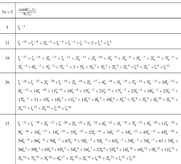
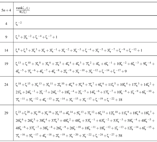
It is not difficult to check from the definitions of the rank and crank that M(m,n) =N(m,n) =0 if|m|>n, so rankn(ζ) and crankn(ζ) Laurent polynomials. Although not immediately obvious, parts (1) and (3) of Stanton's conjecture are refinements of the theorem that the rank is evenly distributed modulo 5 and 7 and the crank is evenly distributed modulo 5, 7 and 11.
Unimodality
Below we will see that this lemma together with Theorem I.4.1 will show us that the quotient in part (2) of Stanton's conjecture is actually also a Laurent polynomial. The reason we said that the fixation is almost unimodal for a fixed fixation that M(n−1,n) =0 and M(n,n) =1.
Log-concavity
In other words, the conjecture simply states that the ratio of consecutive terms forpk(n) is decreasing. Recall from (I.15) that this corresponds to log-concavity as long as it is true for alln>.
Modular forms and Jacobi forms
Therefore, it can often be convenient to find Jacobi forms to find stress sets for modular forms. However, we will only need the sum-to-product identity above, and we are mainly interested in the fact that the root systems yielding weight 1 Jacobi forms describe almost all Jacobi forms of weight 1 [49, Theorem 12.2].
Analytic number theory
Much of the interest inζ(s) derives from the relationship between its zeros and prime numbers. Furthermore, finding bounds on the real parts of the zero in the critical band can be directly related to giving improved error terms for the Prime Number Theorem [33, Chapters 17 and 18].
Algebraic number theory
Hardy [50] was able to prove that infinitely many zeros lie on the line ℜ(s) =1/2, while Selberg [85] was able to show that a positive part of all zeros must indeed lie on this line. This is one of many extensions of the Riemann hypothesis to other zeta functions, and because of the connection between the zeros ofζK(s) and studying prime ideals ofOK, we are interested in studying the number of non-trivial zeros ofζK(s) ).
Summary of Results
The results of Chapter V provide an effective version of the results of Griffin, Ono, Rolen and Zagier [48] concerning the zeta Riemann function ζ(s). The final chapter provides a study of the multiplicity of non-trivial zeros of the Dedekind zeta functions.
Maps from t-cores to sums of squares
In addition to proving other bijections, such as those from Propositions II.2.2 and II.3.1, we also find an explicit mapping in Theorem II.3.3 between the 4-kernels of 7n+2 and the self-conjugate 7-kernels of 8n+1, providing an explanation of Bringmann's observation, Kane and Males [19]. Furthermore, we can use Theorem II.1.1 to prove a generalization of the result of Bringmann, Kane, and Males in Theorem I.2.4.
Structure theorems and relationship to class numbers
However, we are able to combine representations of 4-nuclei and self-conjugated 7-nuclei in an interesting way. However, we can identify this as an explicit bijection of certain 4-nuclei and self-conjugated 7-nuclei.
Combinatorial maps between t-cores
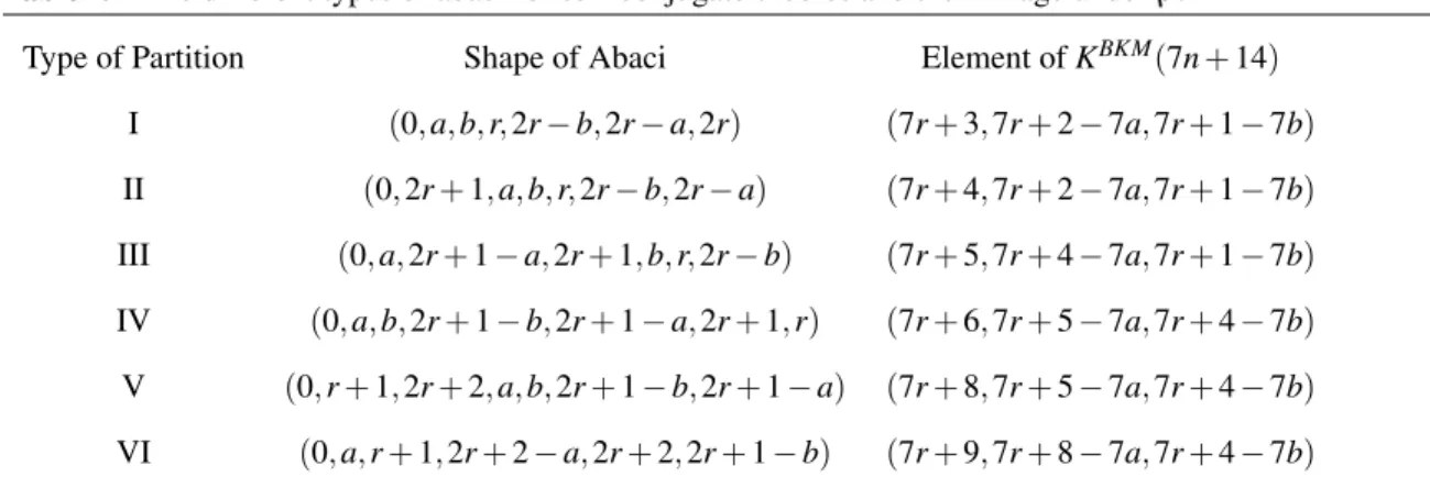
By changing the signs of the first two entries and swapping them (which we can do up to the equivalence ∼OS), we get the result. However, due to the almost identical nature of the proofs of the other cases, we will only simplify the details for type I partitions.
However, as mentioned just before Theorem I.2.6, this is in bijection with p(n), so we conclude that. A well-known result [44, equation (2.1)] is that the left-hand side is a generating function for |Ct(n)|, which completes the proof. Furthermore, we note that the momentums from [18] given in (III.3) below appear to satisfy a Stanton-type conjecture, namely Theorem III.1.5 (this is presumably due to the assumption of Conjecture III.1.4 ) .
Statement of results
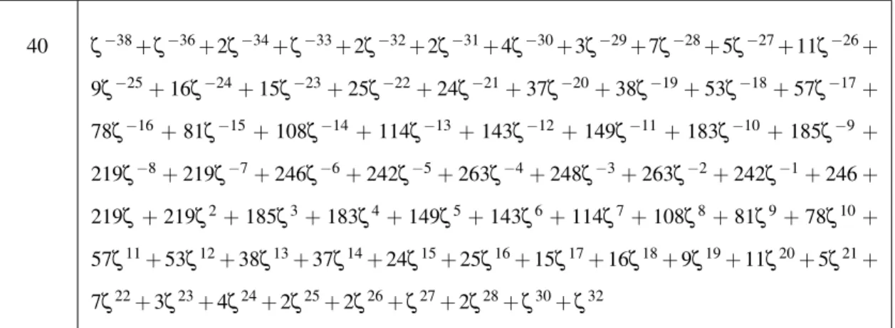
Since we will define a similar crank type in Section III.6, we first define a general notation for crank products that will be useful throughout. However, the benefit of considering the levers of (III.3) is that they seem to satisfy Stanton-like assumptions, while the levers of [83] do not. The importance of Theorem III.1.5 is that, like Stanton's conjecture, the non-negativity of the coefficients hints at the fact that there may be combinatorial objects that count the coefficients of a quotient, which would hopefully provide explicit bijections between sets of even partitions defined by levers.
Proof of Lemmas I.4.3 and I.4.4
We find below that these generating functions provide combinatorial explanations of the congruences of Theorem I.3.3 The cracks of [83] were defined before the above family of cracks and also provide a combinatorial explanation of the Ramanujan-type congruences of Theorem I. 3.3 . In fact, similar to part (1) of Stanton's conjecture, we are able to prove this conditional if we assume unmodality of the coefficients, for which we have computational proofs. This conjecture is analogous to conjecture I.5.2 from above, and [18, Section 4], we provide explicit computational proofs for a more general conjecture that applies to unimodality of the coefficients in (III.1).
Proof of Lemmas III.1.2 and III.1.3
If we consider separately the cases when r is odd and r is even, we see that this is equivalent to the desired (I.13). Furthermore, notice that since f(ζ) = f(ζ−1) we must have cm=c−m, so given the unimodality of the coefficients of f(ζ) we conclude that cm≤cm−1 form≥1. In other words, by unimodality we can conclude that cj−k`−cj−k`−1≤0 for all such, from which bj+`−1 follows.
Proof of Theorem III.1.1
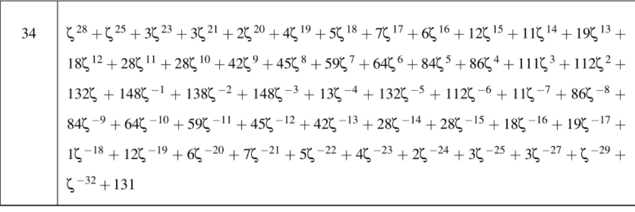
Although we can prove a result analogous to Lemma III.4.1, we will instead make a direct argument. We wish to prove that the conditions of Lemma III.1.3 hold for crank5n+4(ζ) polynomials. We now turn to the proof of Theorem III.1.5, which will also use Lemma III.1.2.
Proof of Theorem III.1.5
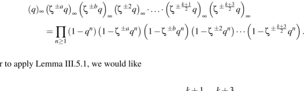
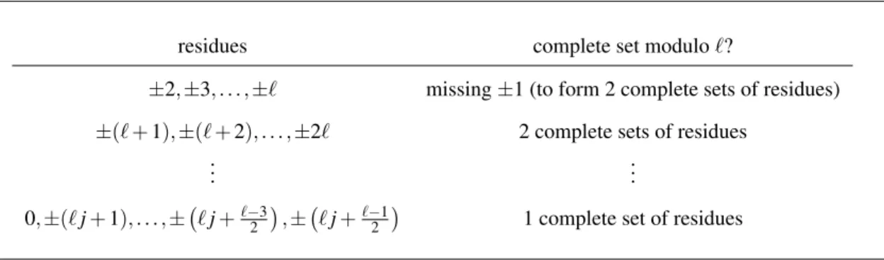
To apply Lemma III.5.1, we would like the powers ofζ in the above factors to fill in complete sets of residues modulo`, that is, we want. To obtain the right-hand side of the claim, we factor outq127 f(ζ) from (III.33) and rewrite the remaining terms as The main difference here is that we had to use Lemmas III.5.2 and III.5.3 to prove divisibility by Φ`(ζ).
According to (III.2) and (III.3), Ak(z;τ) and Bk(z;τ) are products of functions of the form C(az;τ) for different a∈Z. Finally, the divisibility of the coefficients is given by Corollary III.5.5, so the proof of the theorem is complete by Lemma III.1.2.
Other cranks for k-colored partitions
As we'll see below, this turns out to be quite tricky; our primary goal is to find an error bound that holds in a region that depends only on (and not well) Theorem IV.0.1, and ultimately quite a few terms are needed in the expansion of our Bessel functions to achieve this. However, once this is achieved, we can find that the asymptotic in Theorem IV.0.1 is positive, allowing us to make partial progress towards Conjecture I.6.2. Finally, in Section IV.3, we explain how to obtain Corollary IV.0.3 using computational tools.
Explicit Bessel function bounds
We now plug the non-error terms of (IV.7) into the integral (IV.6) and rewrite the integral as a difference of integrals to obtain. If we plug these terms into (IV.6) and then (IV.1), we see that they contribute the terms. If we plug it back into (IV.6) and (IV.1), we see that the second integral of (IV.9) contributes at most.
Proof of Theorem IV.0.1
Isolating the main term
Delimitation of the remaining terms in the second and third lines of (IV.35) is very similar. We now illustrate how to tie the first term in the fourth line of (IV.35), namely. Combining this bound with (IV.34), we find that the expression we started with (IV.17) can be rewritten as.
Bounding the remaining terms coming from Theorem I.1.2
Note that this divides all terms of the productpα(n−1)pα(`+1) into classes, except for the term considered in (IV.17). Combining the limits of the two expressions on the right side of (IV.42), we find that. Finally, we apply Lemma IV.2.2 once more to see that (IV.48) is decreasing inαfor.
Computations and completing the proof of Corollary IV.0.3
Similarly, the bounds of the non-main terms for pα(n)pα(`) are almost identical, so we find that the total errors arising from (IV.37) and the non-main terms are bounded by. Our motivation for formulating Proposition IV.3.1 is that Proposition IV.3.1(1) allows infinitely more cases of Conjecture I.6.2 to be proven using finite computations. Previously it was well known that the Riemann hypothesis is equivalent to proving the hyperbolicity of the Jensen polynomials Jγd,n(x)(defined below), and Griffin, Ono, Rolen and Zagier [48] showed for any solid degreed∈N , the Jensen polynomials are hyperbolic forn≥N(d)for some N(d)∈N.
Previous results
For d=2 andn≥0, the hyperbolicity of the Jensen polynomials follows from the work of Csordas, Norfolk and Varga [32], while ford =3 andn≥0, the hyperbolicity is proven in the work of Dimitrov and Lucas [36]. From a combinatorial point of view, the hyperbolicity of J2,npk(x)forn≥N(d) is interesting because it is equivalent to the log-concavity of pk(n)forn≥N(d). In addition, the hyperbolicity of Jd,npk (x) for degrees greater than 2 can lead to more complicated inequalities that pk(n) must eventually satisfy [36, Lemma 1].
Summary of new work
Recently, Chasse [24, Theorem 1.8] related the hyperbolicity of Jensen polynomials directly to zero-free regions ζ(s) and proved hyperbolicity for all such Jensen polynomials of degree ≤2 × 10¹⁷. It is crucial for our proof of Theorem V.2.1 that the bound on Gm(M) in part (2) is uniformly bounded as m,M vary together. It is easy to prove that Gm(M) is bounded on M for fixed m, but in order for the inequality in Theorem V.2.1 to depend only on a constant (and ned), we need a uniform limit.
Previous results
In our work, we provide a similar asymptotic analysis of the pair correlation function for the nontrivial zeros of the Dedekind zeta functionζK(s), which is given in Theorem VI.2.1. Another way of stating this result is to say that at least 2/3 of the non-trivial zeros of ζ(s) are simple. This led to the GUE hypothesis, which states that the imaginary parts of the non-trivial zeros are distributed as such eigenvalues.
Summary of new results
While this is a limit on the multiplicity of zeros of ζK(s), the meaning of what NK∗(T) is counting is likely less intuitive than it is for NKd(T) or NKs(T). De Laat, Pair correlation estimates for zeros of the zeta function via semidefinite programming Adv. Lee. Pair correlation of the zeros of the derivative of the Riemann function ξ, Journal London Math.
The different types of abaci for self-conjugate 7-cores and their image under ρ
Theta blocks φ R of character ε h determined by root systems R (modified for h = 4)
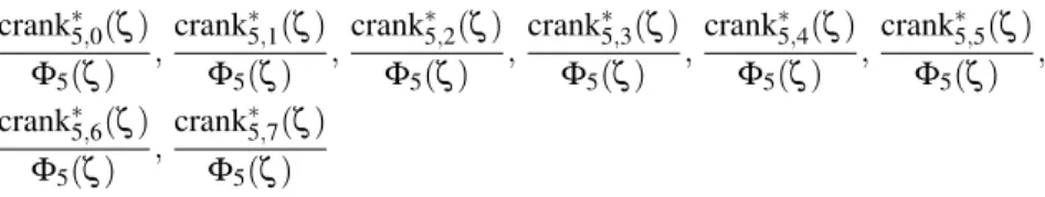
Checking part (3) of Stanton’s conjecture for ` = 5 and small n
Checking part (3) of Stanton’s conjecture for ` = 7 and small n
Checking part (3) of Stanton’s conjecture for ` = 11 and small n
Checking part (1) of Stanton’s conjecture for ` = 5 and small n
Checking part (1) of Stanton’s conjecture for ` = 7 and small n
Missing residues for A k when k ≡ −4 (mod `) is odd
Missing residues for A k when k ≡ −6 (mod `) is odd
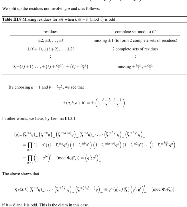
Missing residues for A k when k ≡ −8 (mod `) is odd
Missing residues for A k when k ≡ −10 (mod `) is odd
Missing residues for A k when k ≡ −4 (mod `) is even
Missing residues for A k when k ≡ −6 (mod `) is even
Missing residues for A k when k ≡ −8 (mod `) is even
Missing residues for A k when k ≡ −10 (mod `) is even
Missing residues for A k when k ≡ −14 (mod `) is even
Missing residues for B k when k ≡ −6 (mod `) is odd
Missing residues for B k when k ≡ −14 (mod `) is odd