The relax- ation time and stopping distance are two of' the parai.~eters used to characterize the inertial deuosition of particles

AT BIFURCATIONS IN THE HUMAN RESPIRATORY TRACT

by

Karl A. Bell

Master's Reuort

Chemical Engineering Laboratory California Institute of Technology

Pasadena, California

June 2, 1970

.Rev-ised October 1, ,1970

The prediction of lung disease development in man i'rom aerosol particles and the medical justii'ication i'or subse~uent

control of particulate atmospheric pollutants r equires specific knowledge of the rate and location 'Jf the aerosol deposition in the lun~s. A theoreti cal development is presented to

nvfterically predict the rate and location of aerosol deposition by impaction at the wedge walls in a model of a lung bifurcatior:

IJ."wo limiting flow cases, steady pot ential flow and steady laminar boundary layer flow, are analyzed and found to repre- sent upper and lower bou.,."lds oi' limited experimental deposition data for one-micron particles obtained i'rom a lung appar.s.tus simul ating normal inhalations.

Numerical deposition results for 20, 10,

5, 4, 3,

2, and 1 micron particles in steady potential flow show

denosition fluzes to be i'•.mct ions of Stokes number and also the l oCa1 air velocity distribution along the wedge. Boundary layer deposition results for the same particles are i'ound to corr espond to the fir st few data points

or

^{the steady potential}

case, however no boundary layer deposition oecur>s beyond a

fe1.-.i- particle diamete:C'S along the wedge.

PAGE

Abstract 1

Introduction 2

Theoretical Analysis

5

Lung Model

5

General Streamlines for the Lu.ng :Model 7 Streamlines About the Wedge of the Lung Hodel 13

Tre.jectory Equations

15

Deposition Para.rneter 17

Theoretical Results for Steady Potential Flow 20

Steady Laminar Boundary Layer 23

Boundary Layer Results

24

Friedlander ts Boundar7 Layer Solution 26 Comparison o:f Theoretical Results With Experimental

Results

Experimental Procedure

.~~alysis of Data

Data Fitting ',¹Ti th Stokes Number Smmnary and Conclusions

Ac kn owl edg;men ts References

Appendices

A - ·Nomencla tu.re

B • Graphical Results

C - Experimental Apparatus

D - Friedla....71der' s I:.i1paction Solution

E - Computer Listings and Strea~line Plots

29 29

30

31

33

36

37

39

Findeisen1 in 1935 was the first to develop a theory to quantitatively predict the total deposition of particles in the lungs. In the 1950's Landahl2 and Beec1anans3 have followed Findeisen•s lead with refinements in the equations f'or predicting deposition of' aerosols by inpaction, gr~vity

settlement, and Brownian dif'fusion in difrerent regions of' the respiratory tract.

Their deposition equations are mainly empirical correl- ations which include the basic theoretical relations for settling velocity, Brownian diffusion, relaxation ti~e, and stopping distance (See Table BJ in the ApDendix). The relax- ation time and stopping distance are two of' the parai.~eters

used to characterize the inertial deuosition of particles.

The stonping distance is the distance a ~article travels

before coming to rest when it is projected with a given velocity into still air. The relaxation time is the time period required for a particle to adapt its motion to the accelerating or

decelerating effect of an externally applied force.

The total deposition in any region of the lung is obtained

by S1.1..rmning the separate probabilities f'or deposition by impaction, settling, and diffusion. As an exa~::':;::ile of the er1pirical nab.;.re of these depoei tion equatio:os, La..11dahl ts

for~ula for the probability of inertial deposition is I=P/P+l

where P, the deposition paramete~.e, equals the ratio of the stopping distance to the radius of the bronchial tube. This formula ~,ias chos2n because i t matched the resui ts of an

. ' . , . h

50

^{-,f ' i ' .}

exnerimen"G in wrnc '"'' aepos -cion occurred at a 90 ⁰ bend in a pipe when P equaled one! In all cases, plu.g flow is asstuned, or average stream velocities are used. In spite of the obvious sinrolif'icati,.:ms of these equ.ations, the:v have ':Jeen useful in predicting gross regional deposition rates in the bronchial tre3 and the lower resniratory tract.

Specific areas of ^{the lung} are initially affected ^by some 111ng diseases caused by particle deposition. At these areas the particle de;::iosition rates ^r.iay tend to be higher, or possibly the natural clearing action of the cilia or phagocytic cells may be le.ss effective. Once the natural form and func~ions of these susceptible areas are impaired, the disease rnay spread into surround1ng ^tis c' .. 1e. An exa:riple is the case of lung cancer in humans. Pri::..-12.ry pulmonary

carcino~na in man is considered to b'2 brcmchio:;enic in origin and us1Jally aris.sd in a urinci~al brG..nch of the main bronchus near thB hilus of the lung. It is caused b~ direct primary contact of c2rcinogenic vapors or particles (asbestos, arsenic, chromates, nickel carbonyls, tars, and r~dioactive minerals) on the e9ithelial lining of the bronchus. The ganeral mechanism for tumor develoo~ent is bel ieved to be the following: in

the bronchial lining a defect caused by the carcinogenic substance is repaired by a tra..risi tional type cell uhich -,,ri l l dif.ferentiate normally; however, when persistent injury occurs, they rorrn

Wi th toda:-t s inter est in C:Jmoating l'.i r uoll'-3.tion and

i n model ing the environment in a manner t o optimize the quali ty of l ife, man desires t~ be abl e t o 9redict statisti cally t he chances of his obtaining lung cancer or ^so~s other r espiratory disease from breathing pol luted air containing various gases and particles. Therefore, he must be able to predict the rates of deposition of specific si ze ~articles at specific locations in the lungs. The previously described empirical correlations for regional deposition are inadequate because t~ey negl ect

local variation in stream velociti es and fail to account for the transient momentum and concentration gradients ..

Inasmuch as l ung cancer develops in the main bronchi and its branches, it is probable that some of the particles contributing t o the diseas0 are denosit ed by ine~tial forces since the fl ow r ates arc! hi gh and ths streamlines bend sig- nifi cantly at the bifurcati::>~. The bi..Curcat ion region is, consequently, the f ir10t l ogical ¹¹hot spot¹¹ to investigate in the lung.

The goal of this masterTs renort i s to theoretically predict the rate and location of the parti cle deposition at the bifurcation of a lung model anc to co~pare the theoretical results ·with experimental data taken f'or a flow syst em analogous to the first bifurcat ion in the upper air1-rnys.

Lung Hodel

In nearly all theoretical deposition studies, Weibel's5 regular symmetric dichotomy rr.-Odel of the l u.ng is used. For the author's theoretical study a two dimensional r1odel of the trac~1ea and its two bronchi with a 90° _interbronchial angle

and an overall shape identical to ~'1eibel rs model is proposed.

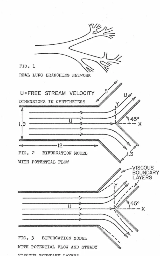
A s>:etch of a real lung branching neti:-mrk is show-.n in Figu.re l;

the model is shown in Figure 2. The two dimensional model

was chosen for study because it simplifies the analytic solution of the stre&-nlines {vorticity effects arise in three dimensions).

This simplification· should remain accurate ·:ror the stre&"11lines cl ')se to and on either side ^01~ the stagnation streamline.

Since gr avitational effects are neglec-cea in horizontal flow, only inertial forces are considered. The 90 ⁰ wedge Has chosen be-« cause it shnnlifies the not en ti al and boundary layer soluti·Jns.

The model is also geomet:t'icall~:t similiar to all branching sections in the ^UD~er respiratory t ract of the lungs; therefore,

denosi ti'Jn predicti::ms for this sect~.on can be .flow r2.te corrected and applied to any other section.

The :main disadvantage is that such a two dimensional sy:rm'":ltric model is n:::it ^s. co::nplete simulation of the three

dL-.en~iJnal :flows in the real lm:1g.. The real ^lu...11r~ is uns:a::.- r.'et:d.c with an interbr:)nchial angle whic'.:-:. varies fr'.::rr:

50

to 100 degrees. The angl e seldom i s bisected by the ~racnea,

REAL LUNG BRANCHING NETWORK

U=FREE STREAM

u

>

>

....

~~~~~12~~~~--l~

FIG. 2 BIFURCATION MODEL WITH POTENTIAL FLOW

>

u

FIG~ 3 BIFURCATION MODEL WITH POTENTIAL FLOW AND STEADY VISCOUS BOUNDARY LAYERS

L3

dimensions. Finally, the outside walls .of the real l ung

trachea join sr.!oothl~: with it s branches in many possible angles, whereas the model has a sharp 135° angle.

An air flow analysis of "ileibsl ts s.; iCTnetric · l u..:."'!g model is 3i ven in To.bl e Bl in the A:puendix. The :8.e~/nolds nlli?1bers

ano the entrance lengths sugge2t that lam:Lnar plug :flow exists in the first through ^{fourt~ g~nerati~ris,} partially developed la.7ninar parabolic flow is present in th:; fifth thro•.J.gh eighth, and well-developed Poiseuille flow takes place in the ninth through fifteenth gen~rations.

For the model studied two flow cases are ^assumed~ (1) stsady potential flow shm·m in Figur8 2 and (2) steady noten- tia1 flow with steady laminar boundary layers in the bifur- cation region of Figure

J.

In the _·'· notential flm-;r solution

the infinite velocities at

13 5°

angle are neglected because t'.0.e :main concern is w·ith the stt'ea'1lines ab:Jut the wedge.

These cases are simplificati:ms of the real lung flow which is nearly sinusoidal in time and 1"-hich c2"uses an unsteady

bc:nmda:~y layer to develop along the tube ·walls. Eoweve-e>,

thess cases are valid starting points for a theoretical analysis.

General St:rea"'i1lines for the Lu:'.ig T:Iodel

Having assw.--ned the two air floH cases, the analytical equations for the steady potential flow will be derived first.

~ . • 1 ^mi 6 • 1 t • ,

~1 ne-1nornson gives a so u ion proceaure for the genera.l pr')blem of determining the streamlines in a ca.:.1al with a side bra...11ch. Since the i'low :model pro-posed above is sy.1.i.mat:ric, the strefl.!.-nlines can be derived by modifying Nilne-Tho:mson' s procedure for either the top or bottom half of the model--

the center being determined by the 8.tagnation stre!:.:mline which t erminat es at the wed~e tip. The top half

or

the madel is shown in the z-plane in The free stre&~ velocity

upstrea..111 from the branch at A₀₀ is U, and the dm·Jnstream velocity is

u

2, unknmm. ACDC is the stagnation strea'Ylline~ t,.rhile the strea'7lline -~ED00 undergoes an abrupt change of direction at E, causing 2n infinite velocity.

First, the branch for~ in the z-plane i 2 eliminat ed by transformir;g into the Q-plane ('Figure

4}

by the transf'orr:;2tion equation

where -1.G

~ =

'7

e =

u.-

i

v •

Here q =

1J ^u.;i. +

y.2 , the stream speed.

Along the sides of the main canal 9

=

^{O; while along the}

branch 9 =~. At C, q

=

O; hence, Q is infinit e. The infinite strip in the Q-plane can now be mapped into th8 pl ane {Fi gure

4)

by means of' the Schwarz-Christoffel transforr,oa ti on, which

(1)

Aro /u2

/ 1Y Dco

&-..

h

.. ;.... u ^I I ^I

Aro Z-PLANE c

e

D O=cJ..

Q-PLANE

I

Dco //////////J.'./// $///////////////Aro

o/=U2h2 \ C) o/=Uh

~ .... 1T u ;

D o/=0

I

o/=O A

co ////7/7////7/7/7//////7/7///7/// · ro

E 'J'J-PLANE

FIG.,

4

The following values of

-5

and 0 correspond by the above

transfor~ation equation:

S

^=-a

-5

= d

~

= u

"'. 1·nere1ore, " J_rom -<> (J) _ a= ~ J.., c."na· a.· -- (r.~1·-,..-_....,;-ur)¹~

The next step is to construct the com~lete

1 ; ^T 1 , T.

p ... ane or v'i-p ane i·.rnere N

=

~ +

i¥.

^<f> represents

n .t.. • , • ~ 11r ·, ' ' h ' ^{.c>- • •}

1uncvion, wai.Le ₇ represen-cs ^'C _e S'Crea."'11 1.Unc-cion.

(2) note11tial

the notential

boundary conditions are as follows:

on ^P.J.00EDb?

on AwC on GDco Therefore,

lf

=

1V =

Uh - U h - 2 2

1JI

⁼

0 Uh u_2h2

which also follov-i2 fron the equation of Cr)ntinui ty ..

( 3)

cµ1d ~

=

^{-()0 at Doo, the} result is the H-plane diagram sh::nm in Figure ~-· To map the ".I-pl2ne into the

..5

^-plane, the Schwarz-Christoffel transforl¹-:ation is used 2.gain, and the result is tirn following:

Integrating:

- I)

I

^{K ,. · { P -o}

\A (CJQ d'l---

V\ --:: (;;:+d) J (S

+-u)

⁽⁴⁾

The auth·:>rts origins.l potential flo",,i derivati0n ::ras

critically a.n2..lyzed by D-t' .. lforman ~¹~a1-nPth a~'!:i Dr. -.Ii ll iam Eal1. 7 _They found that :Milne Thomson rs

de ~' i

vatic>n and sub-

sc;qusntly ny ?)revi·:>us de'.'i vat ion uas in error!' because K 1 and L

1 ^1:rn~c-e a::: su:med to be either real or irr::aginary 1-rhen applying tha boundary conditions to evaluate K

1 ^arid L 1 ..

As indicated above~ K

1 and L

1 must both be assumed to be comnlex constants in order to be evaluated correctly.

Using the boundary C·')ndi tion that

If=

^{0 on DcoE,}

Cb+

a) and

(5 -

d) have the same sign.. Thus· on D°"E the logarith.'":1s are all real- Therefore on D E _"()Q

Cp -

Ther·efore,

.lm

L1 ::

-Im I{, 105 ,~ {

la. +-d )

t

^+a.

Evaluating the log in the ^' limit as Re ...!J ^p approaches()O , Therefore, Im L1 ^{= Og} Thus

0

=

-Im I<, /oCt ^1· ~ -J 1·

log (l)= O.

(CL +. d ) J

t

^+-a.

..~v· ,_., al atin u· ,_ g '-'ne lo ^0. g i·n • '"'· +-h e l _li,l'C ·m· · a S.J·,, f...:...o , _~, ^o:z..· .:,

J-}J=

..,,. C·v",.,_sran.t,· .. , ...

therefore Im K

1 =

o.

Applying the other boundary condition that¥=

u

₂h2 at

c,

set

¢

^{= 0 since C is a} stagnation point.

ThusJ= Oat C.ar.d substituting into (4)

F^~_om .- ^~v•h_e _ resu_i:;s 1' Of ~h u e 1.lI'Su ~· '- -cwo ' b oun.._._c..ry ~n C'~~a0""' '~r·on~ J . v l -··-·

the last two terms equal zero. Rearranging UJl\_{1 (} a+d) _

T/

above1

Using

cf;=

O,

O= - ^.~,/

J/k,

0

There.fore

Substituting these values of L

1 and K

1 into l4) and setting a

=

^{1 from (2)} the general solution for the complex potential in the symmetric model is the following:

- w:; ~

^/OJ

IJ'/J - ~

11

! +

I From (1)

Theref'ore

{ _i )

'Yo< _ {

-vljei.,,<) 3

$

-= -

u - \

- ^~

_{dz -}

- ^~ ::: u

^e-Loi.

^s1'rr

Differentiating

(4')

and dividing by

(5)

the result is d

z :: - ~ ^[

^{I - _J_}

J ^e

^{i o<}

^{Ji - -</11}

J

.S ^7T (~ ^-cl) (J +

I)

( 5)

Integrating 1:1i th respect to

J

^{with o<}

=J!j

^{for the} 90° riodel

7

= -~ ^{J. %[ f J-Yt; JS -} c_r ^{J5j 1}

L n

S-d J t+1

Transforming variables by

S

⁼

x4,

evaluating.integrals from tables8 and substituting d = (h/h2

)4

^{from (2) and} (3) above, the

z=

(6)

Since z

=

0 corresnonds to

.S =

0 from the transfor:nations in Figure

4,

the integration coDstant C =

o.

Because (6) is not invertible to give

J

^{= r(z), one}

must use both (4') and (6) as the solutions f'or the complex notential at location z i.n the z-plane in terms of' the implicit variable

.5..

^{The stream} fUt.-iction ~ is the complex part of Td in terms of

.J

at location z in terms of

J .

^{Likewise, the}

complex velocity

0

⁼ u - iv is given by

(5)

in terms of~

at location z in terms of Sin

(6).

Therefore, derivation of an analytical expression giving the stream f'unction or the complex velocity as a direct function of a z-coordinate position is not feasible .

. Such a pro bl.em should be solvable numerically on a computer. The procedure to determine the stream function, for instance, would be to feed the cor.rputer dif'f'erent values of the com~lex variable

J'

^{and to have i t calculate the z}

coordinates and the value of the strea.."'n function

1(

corres- ponding t'J each value of.£. Then the co:nputer would sort

thro'.;gh this data for all the stream functions of one value

and store the (x,y) coordinates of .that stream function. In

orde~ to plot the strea~lines in the z-pla.~e for each value of

?f,

the coordinates would be arranged f'ron ninimur:'l to maxir.m::n based on the x coordinate.

To . ^.... .

aeverm1ne the strearn velocity co::nponents at any co-

·'Jrdinate locati on in the z-nlane, the cozr:puter wou.ld like- wise use different value~ of~ to calculate corresponding values of u + iv and x -:- iy, <:·1hich w:::iv.ld. bs stored in arrays.

T~e nTu~ber of different points in any are.a of the z-ul ane is in:finite; there:Co:'.'·?,, one sh·J'J.l d try to choose values of

J

to obtain values of (x,y) ~hich are equally distributed to the acc·'..J_rc:.cy desirsd over the range of the z-plane in which one is concerned. Thsn at any possible point in the range of use on the z-plane, a value of u and v ce.n be fou.."rJ.d in ^t~l.e stor-ed arrays.

Values of ljf have been comnuted at various (x,y) coor- dinates by using the procedure described above. However, preliminary results indicate that the ^~11ount of computer

time necessary to do an adequate job is presently prohibitive.

In the case of aerosol de:oosi tion, the streamlines ·which lie close to the stagnation streamline are of princii;ile interest because small particles on strea~lines i'ar ^.f'l -'-rom i,ne ^{.?.. "I} s-cagna-cion ^{• • •} streamline in the direction of the channel walls will neyer impact on the wedr;::e. This is clearly demonstrated by the fact that the Etopping distance of 20 micron particles in a stream having a velocity of 100 cm/sec is only about .087 centimeters in the direction perpendicular to the wedge. Since 20 micron particles are approximately the largest particles to penetrate beyond the nasalpharyngeal chamber, all smaller particles

that imyact on th-::: wedge will have to travel on streamlines lying within

.087

centimeters of the stagnation streamline.

Therefore, an approximate solution is desired for the strefu~-

lines about the wed~e b;y expanding the gene-cal solution about

J

⁼

o.

Streamlines about the Wed.R:e of the Lun.~ Model

3xpanding the comulex potential (4'} in an infinite Macl aurin Series for small~ and neglecting the second and higher order terms, the result is as follows:

Therefore, .

~ ~ U~

^[-

(J_

^{+ I \ ]}

d :$ . _TT d )

dZ

=

^{dW/JS::: }:_}

^{e..io<. .:5-~?r(f} +-/)

d ~ J W/JZ Tf ·

Integrating with respect to

1

and setting the integration constant equal to zero since z

=

^{0 when}

J

⁼ O, the result is

z

⁼

Choosing<>< =

-fj,

solving forJ, and substituting .for the constants, the

Theref or-e

.,... I W _ ^-(.'IT

~-Ue-;:;

d z

The constant,

U YA

;;, [(~i)i+ if~

u_-i\J

represents the value of u at z = -1 and is designated by

u_

₁•

By use of the approximate equation and substituting f o r j W ;:

-~

^[

~Tl

^{- (}

d +/) S]

W - _- - _-Ji

^{7-. I}

u_, ^e

-~ ^o/3

^z

^{if/3 .f-l}

u

^{ri I}

(7)

Using (7) in polar coordinates for flow around a 90° wedge with the orL2'.in at the wedge th) and ·with r =

V

x:~ -1-

'IJ.

^{7 ,}

9

=

arctan y/x,

:i I)

% cTi-fe)

~

-:: - lq

^··I r cos

3

y-::: + ~ U_, /f3

^{5111 (}

rr;'IP)

^-1-

uA

₍₈₎

(9)

·· · L) '

Y: (

TT-9)

v = _

₁

r

3 sin.

3

⁽¹⁰⁾

(9) shows that the u velocity component decelerates toward the stagnation point and accelerates along the wedge. The v velocity component in (10) is noted to continually increase over the saue range. These results are directly applicable to the z-plane since theJ dependence has been eliminated.

Tne California Institute of Technology IBM 360 computer was used to plot the stre8..:."11lin2s given by (8) about the top half of a 90° wedge shown in Figure El in the Appendix. The free stream velocity was taken as 100 cm./sec., which represents the average flow rate of a one second JOO cubic centimeter

inhalation through the lu.i"'lg model.

u_

₁ is, therefore, equal to 81.97 cm./sec.

1jf = 95

represents the stagnation stream- line or negative x-axis, while

lf=

^93,

'lf =

91, ... ,

1V =

⁷⁵

represent values of the stream functions on the successive streamlines above the negative x-axis. As pointed out earlier the 20 micron particle, the largest particle studied in the subsequent impaction an2lysis, has a maximur.i stopping distance;

8 _;:;

.?XlO - centimeters, perpendicular to the -:·;edge. Tb.ere fore, the only streamlines needed for the theoretical impaction

analysis will lie under

1f =

90. Because the abrupt

135

^{· o} bend in the cha..Dnel lies at a distance of l.J centimeters perpen- dicular to the wedge, one can readily assume that the ini'inite velocities developed there will have no effect on the streamlines close to the wedge. Since the general solution streamlines,

if they were obtainable, wo;Jld have the sane shape in the region close ^to the stagnation streamline ^and w:3dge surface, it can be assumed that the anuroxima te solution s trea.-r:lines are sufficiently accurate for this calculation.

Trajectory Equations

Havi!lg obtained equations i'or the fluid velocity in the model, one must develop a method to apply particles to these streamlines and to determine the rates and locations of their

·deposition on the wedge wall.

For particles ranging from one micron to 20 microns in diameter in a 100 cm./sec. stream, the particle Reynolds numbers ranse from .06 to 1.2. Stokes Lm·r, Fk =

6yRu

is valid for Re up to .1; while at Re

=

1, it predicts a drag force which is 10 percent too low. Here Fk is the force

associated with the fluid stream movement,/ is the viscosity of the fluid streai.:i, R the particle radius, and U the free stream velocity(lOO cm./sec.). In spite of this error with the largest particles, the author will use the following differential equations of motion for particles within the Stokes flow regime:

J Ur= .1.(U-Llp)

J t

1:

u and

v

are the stream velocity components in the x and

y

directions, and liD and VP are the particle velocity components.

1:', the relaxation time of the -oarticle, is ec:uivalent to

Fk/mass of narticle. The technique for determining the aerosol particle trajectories in curvilinear .flow is outlined by

Fuchs9 and consists of dividing the trajectory of the particle into corres-ponding segments using the approximation for the i-th interval:

d ur __

-rt

where ti. is the value of ti at the beginning of the interval.

1

Integrating and assu."ning t = 0 and

u ..

= U: • gives

n pi

. . -t/'"C"\

llp =-Up"

+

(u.~ -llpi.

)L / -

e ^{J (11)}

at the end of the interval and integrating again gives the x coordinate of the particle at the end of the interval

I ( ) (

--1::/i:)

X "" X

~

+

^ll;_, ""C

-+ '(:

^{tip: - f.Ll, . I -}

e

(12)

Calculation of a trajectory in the model will begin at one centimeter before the wed.:ze where the stream velocity is essentially rectilinear and equivalent to the free strea.~

velocity. Therefore, the particle velocity ca...Yl be assu."'iled equivalent to the stream velocity Ht this point. Our stream velocities u and v are given by equation (9) and (10) for all points through which the particle can pass. Beginning at x = -1 cm. where U _p

=

^tt, the trajectory is calculated step by step by -use of equations ·(11) a.."'1d (12). Obviously, the accuracy will be improved with shorter time intervals for each step in regions c16se to the wed~e where the stream-

lines curve significantly.

Deuosition Para~eter

How that the equations for determining the trajectory of the particle have been derived, calculation of the posi- ti::m of the particle will continue. until the particle con- tacts the wedge surface or until i t travels beyond

2.5

centi- meters along the wedge, in which case it will be considered

to follow the f'luid streamlines. The general deposition

uara~eter to be ~easured, F

3/C, is the flux of particles to the ·wedge surface diirided by the concentration of particles in the stre&"'11; it has dimensions of crn./sec. This is related to the flux of particles in the main stream, F

0, by the principle of continuity, F

0dy = F

8dL, where dL is a small segment of' the ·wedr;e surface at a point L fro::n the wedge tip.

In order to apply this to a finite nu.i.~ber of particles

colliding with the surface at a finite nu..mber of positions, the equation, dy =by

=

^y₂ ^{- y}₁^{, where y}₂ ^{and y}₁ ^{are the}

vertical starting coordinates of two identical particles at x

=

^-1 centimeters, is used. These par1..oic_r.^{.I- • ..,} es ir:uact at 12

and Ll ^{on the \.,red,-:e sur~f a.ce with an} ave::."' age deposition location of (L

2 + L

1)/2 and dL =D.L = L

2 - L

1• Therefore,

Fs/c :: (Po Ii Y)/[c ^{LlL) = er.}

^cosG

{/1,Y)/(11 L)

whe-C"e q is the average speed of' the two streamlines at the

two starting positions y₂ and y

1 and 8 represents the angle bet;-reen the average velocity vector and the horizontal coor- di::late. This deposition for:nula ca.."! be -c:_sed acct~rately if all -:>articles are started ^T,-fi thin the same small y distance

of each other. To ^dete~mine the ^nu::~ber of ^particle~ depositing in a neriod of time, multiulv _{~ ,} F /C _s bv _v the u_" article concentration in the stream and the period o~ time of deposition.

Having derived all the necessary theore'.:-ical equations, a program was wr itten for use in the IBH 360 computer to determine the deposition rates · and loc2.tions for aerosol particles in st eady potential flow. The Fortran IV progra.11 listing is given in Appendix E. The variable inputs are the free streari velocity, particle radius and relaxation time, the y increments between starting positions, and a time inter- val. 20, 10,

5, 4,

3, 2, a.nd 1 micron diameter particles were run because the 20 micron particle represents approxi- mateiy the largest particle size which penetrates beyond the nasal pharyngeal passages' wh-:reas the o.ne micron particle is essentially the smallest particle having a. relaxation tir.ie long enough to imoact on the lung walls.

In order to approximate the deposition that occurs in

the unsteady flow of a real lung inhalation by using the steady flow computer program, the quasi-steady flow approximation

is applied. This approximation holds when the dimensionless parameter

R1W/~:

is less than 1.010• R represents the radius

of the main tube before a bifurcation,W represents the angular breathing .frequency, and ...J1 the kir.ematic viscosity of air.

In other words, the unsteady periodic velocity profile r,.;hich occurs in the resuiratory tract upon inspiration and expiration can be treated as a time succession of steady state velocity profiles when the dimensionless frequency parameter has a value

less than 1.0.

Table B2 in the Appendix shows the -v-ariation of the frec_uency para.r.11eter in the upper airways for breathing rates of 12,

16.7,

and 30 breaths per minute. The values of the parameter are less than one for the three frequencies used in the 4th generation and proceed to decrease to values of .08-.13 in the 16th generation. In the trachea and the first three generations the value decreases from

4.14

to 1.22 at the 30 BPM rate and from 2.61 to • 77 at the 12 BP1'¹I rate.

The author's bifurcation model has dimensions of the first bifurcation bet·ween the trachea and primary bronchi. Since the frequency parameter for the three breathing rates varies from 2.61 to 4.14 in this region, the quasi-steady flow assi..unp- tion can not be rigorously assumed. However in order to

sinmlify the task of predicting the depositi on, quasi- steady flow will be assumed as a first approximation.

The following technique was derived to apply the quasi-

' d "'l t . . . ^{1 • l ' •}

s0ea y I ow assump ion i:;o -c.-ie aul:nor s cor::,pu--cer program. The cam design curve, shm-m in Figure C3, approximates the f'low rates for a one second JOO cubic centimeter breath. This has been divided into 16 time intervals, and the average

flo~·i rate has been calculated from each interval by sta..ndard tech..11iques. Table Cl lists the average flow rates and average stream velocities calculated. Then the above computer program is run for a single particle size repetitively at these differ- ent average flo-,, rates. Eean values of the deposition flux are calculated at· a_ fixed -.loc.ation along the ·wedge by ·weighting

the deposition flu..."'t at that location for each steady f'low rate run by the aDpropriate time interval; all the time

t-reighted values of flux are then sw'iimed to :::--i ve the mean value.

Theoretical Results for Steady Potential Flow

A plot of the trajectories of 20 micron particles in 100 cm./sec. potential flow is sho·w-i:-1 in Appendix E2. In

order for these particles to impact as shm·m, they are started at x = -1 centimeters, senarated ~ertically by

40

microns, and a time interval of .0001 seconds is used with a relaxation time of .00123 seconds. At the more accurate time interval of .00001 seconds, used in all subsequent results, the maximum extent of impaction for 20 micron particles is

1.5

centimeters downstr·ea.l71 of the stagnation point,. This result is obtained from a vertical sta"!.'"'ting position of .02L~ centimeters~ which is slightly more than one-fourth of the stopping distance

calculated with 100 cm./sec. flow. These results clearly show that all particles rmst lie within a fe',.J diameters of: the

stagnation strea:.-:¹line in order to inmact on the wedge.

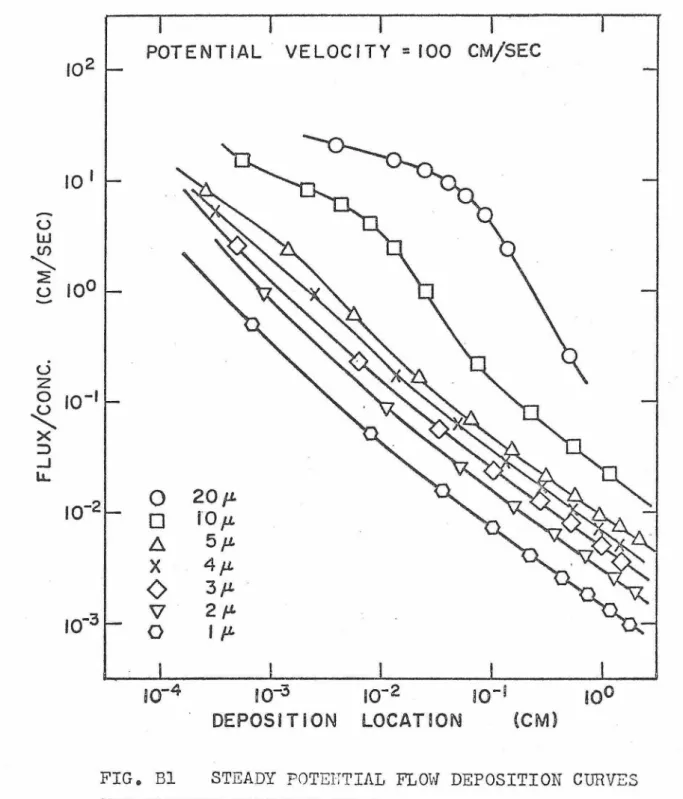
Table Bl lists the relaxation times, stopping distances at 100 cm./sec., and the y starting interval between particles for all the particle diameters ^r~m in the results belmr.

Figure Bl is a plot of log F /G vs. log L. The 1, 2, s

J, 4,

^and

5

micron plots are observed to be fairly linear;

their nearlv constant seuaration is an_"-' ""- ... nroximatelv ' v related to the log of the ratio of their relaxation times or diameters squared. Hmrnver, one notes incre2singly nonlinear regions

from the L~ micron to 20 micron particles at loc.s.tions increasing

-3

-1

respectively fro2 10 to 10 centimete~s. One also notes a hi~her dBnsity of deposition points in ~hese regions for the 20 micron and 10 1nicron particles. One naturally expects the decelerating and accelerating effec~s of the potential

velocities to have the least effect on the 20 ~icron particle's motion and increasingly greater effect on the smaller particles.

Therefore, the 20 micron particles easily traverse the slow velocity, curved strea'l'lline region near the tip of' the wedge with little deflection to impact directly on the wall. Th.e

same can occur for the 10 micron particle, but at a distance

!""'our times closer to the tip to insure negligible def'lection from its original path before the wed~e. This reasoning is carried on closer and closer to the tip for the smaller

uarticles with sh'.Jrter r elaxati::n1 times, thus explaining the shift and decrease in size of the nonlinear segments of the plots.

Since the computer pro:'!r am is designed to terminate the trajectories when the center of the particle is less than or equal to the particle radius, th8 size of the radius causes a small part of the effect described above. If the particle falls beneath the imaginary boundary, the calculation of the exact deposition location is ba~ed on the radius.

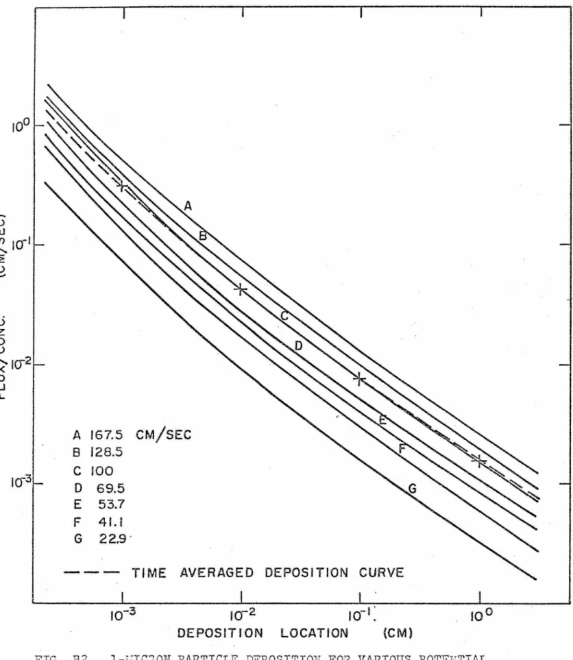
Figure B2 shows the effect of various potential flow

rates on the deposition of one micron particles. The velocity averaaed _b deuosition curve marked wi~h crosses is determined by the tecJ:i..nique described abJve to approzimate the unsteady flow rate dspositi~n of a 300 cc, one second inhalation. Since i t nea!'ly coL1cides with the 100 cm. /sec denosi t i on curve, the

100 c~.

Is

ec. steady potential deposition r '"'sul ts ~-rill be used to approximate 1.:nsteady flG¹--r resu_l ts. All t>e ^c:~:rves have t(le sar:!e shaps, indicatinr that the main ^efl~ect of vary- ing the velocity for the one rnicron ~articles is to change the value of the coefficient of the deposition flux term.

Because of the small particle mass and relaxation time, the inertial effects are very small causing the uarticle to deviate only slightly from the streac""'ll ines. The:r>efore, the nonlinear regions ^fo~nd for the l arger uarticles do not occur for particles smaller than

4

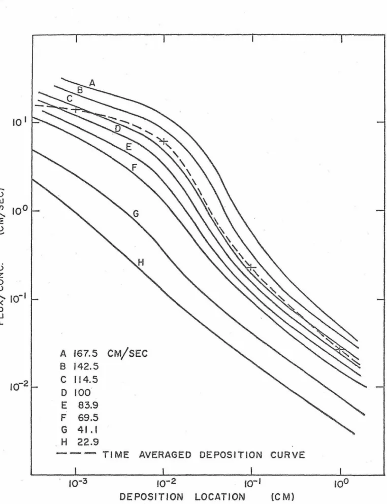
microns. Sum ... ~arizing, inertial effects cause negligible change in the deposition flux for one micron particles T,-;hen various stream velocities are used.

Fig-u.re BJ fol"' 10 micron particles is analogous to Figure B2. The higher velocity plots clearly show the nonlinear portion explained in the first gr a9h. Higher velocities are naturally expected to emphasize the nonlinear portion while minimal effects occur for the slowest flow rates. This is because tha degree of deceleration and acceleration is much smaller than at higher velocities, causing the particles to follow the streamlines more closely. The maa.."11 denosition curve to be used for the unsteady ~ flow auproximation .:.. ... corres- ponds ap9roximately with the 114 cm./sec. data instead of the 100 cm./sec. data. This shift in the mean deuosition curve is due to the increased inertial effects for the higher flow ,..,a ... ⁰ riuns T.Tbi cl"' o•·tt·re1 ah

- .. v v .... ~ .... _ .!..L .... J.. , - o the effects of the slower runs.

Steady Laminar Boundary Layer

Having s·Jlved the inviscid flow case, a steady l&'Tiinar boundary layer is now added along the wed~e to determine its effect on deposition. The potential solution for the flow along the wedae from (9) and (10) is

ub ::: ^{u_I ( ;J :::: u_ (}

^XbYJ

The boundary layer coordinates are xb and yb, respectively parallel and perpendicular to the wed:;::e sur ·~ace. This is used as the limiting velocity above the bovndary layer along the ·wedge.

""' S hl ' ' t. ^I l l d • • - 1 . n 'h 1 . t

~rom c~_icn ing s imensioniess ^{p_o~s OL ~} e ve oci y

. 0

distribution in the laminar boundary layer along the 90 wedge, one determines the boundary layer

b'lX) =

3. L/3

Hr/u_,

¹

^{X {}

³

thickness at u,/U

= .99

to be

0 .

Another approach is to use the displacement thickness12

t .I ' · ~

~ C«) :::-

^{I 95"S}

v-->(u_,

^Xb

as the b·'.)undary layer thickness.

A cubic eauation was found to be a poor approximation for the bou,.~dary layer velocity profile by the Von Karman Integral r,lomentun1 Equation. Thererore after applying

Schlichting's dimensionless parameters a series expansion of the velocity profile for the 90° wedge was obtained f'rom the

· · 1 +-·cl -" Fal' ^{,:> ,} 31 13

or1g1na arvl e Ol KD~r ana Kan • The comuonents of the velocity in the boundary layer are therefore:

[

(U-1)

fl~

.. ( U-')·

^{i -~}

Ub :::

u_, :s Ti

^{fb - • 100}

Ti Yb xb

In order to deter~ine the denosition rates with the

steady 12.lllinar boundary layer, the s&--ne basic co:r.:iputer ::crogra:m is used as in the steady potential flow case. Eowever, the boundary layer thicloess is applied as a boundary condition for switching the particles from the potential :flo~._. equations of motion to the equations of motion based on the b01.L'1dary layer velocity components. The ^sa.~e denosition par8.I:1eters

.. .

are used. ·The Fortran IV program listing is given in Appendix l

T'ae displacement thickness was used to obtain the reported data below because the other boundary layer thickness equation gave essentially identical results for all particle sizes.

The dii'ference between results was negligible because all sizes of particles which deposited on the wedge entered.the boundary layer well within the maxi:mu..ll thickness predicted by the displacement thickness equation.

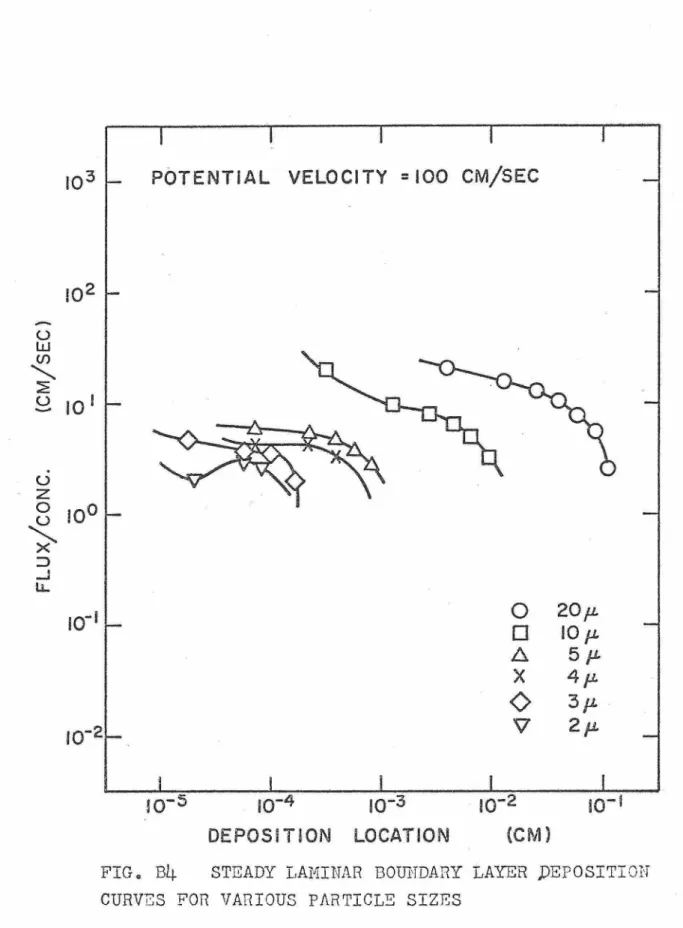
Boundary Layer Results

Figure

B4

is a plot of the deposition results for all particles in a 100 cm./sec. potential velocity stream with a steady viscous boundary layer on the wedge. As one would expect, the slow viscous boundary layer tends to quicxly dissipate the momentum of' all particles entering it. Only the large 20 micron particle is ca~able

or

penetrating and deDositing at a maxirmxm distance of .1 centimeters from the wedge tip. The 10 micron particles almost reach .01 centimeter and the remainder of the particles are all deposited -..Ti thin a distance equivalent to their di&'!!eter from the wedge tip.

The curved tails connect the f'irst denosition Vf:.lue along

the wed~e with a theoretical denosition value at the wedge tip, evaJ.uated ^{wi ... • -1-l} n L

=

^{10-6 centimeters .} Deposition plots within 10-4 centineters of the tip are theoretically possible but realistically meanin.cdess '.-rhen dealing with particles

larrrer than 10-4 centimeters. The plots f'or 2,

3~

and

4

microns dip before taining off because the average de~osition location is bases on a deposition at L

=

O and L == twice the average location.

Comparisons of' this graph ·with the steady flow case of

Figure Bl show that the b·'.)undary layer plots roughly approximate the first deposition points of the steady flo·w case f'or the

4

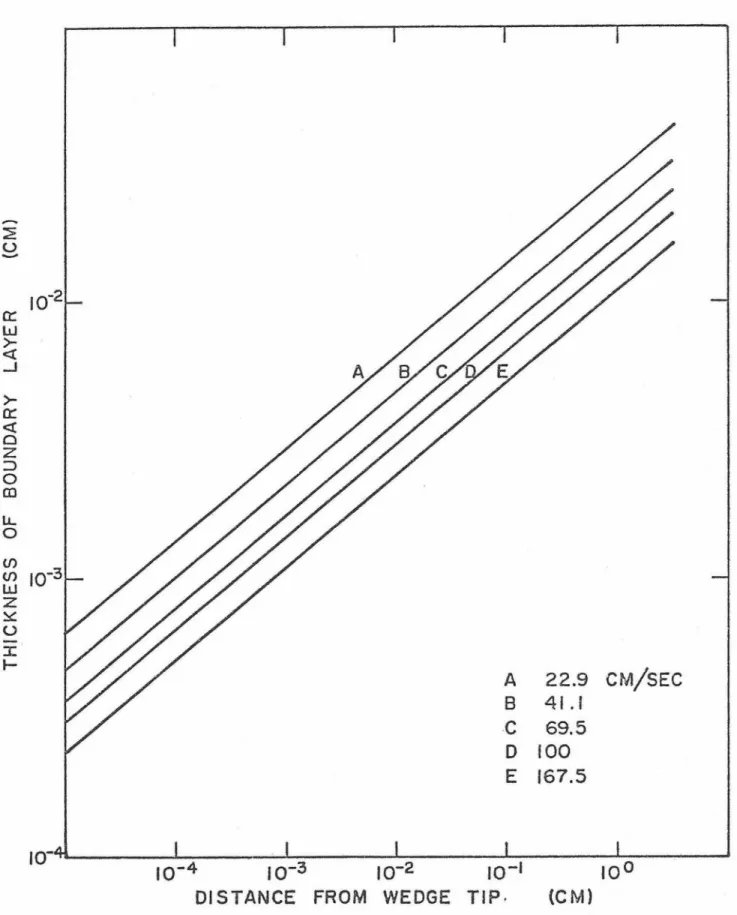
^{micron and} larger particles.

Figu2"e

B5

represents the steady bou...n.dary layer thich."Tiess for different steady potential velocities; The thinner boundary layer at

167.5

cm./sec. indicates that more deposition will

be possible than at 100 cm.;sec. but that the thicker 22.9

I . 1 ~ +' th h. , ' ...

cm. sec. ^{case wi_.l .Lur __} er _ ino.er ae:::iosi1,,ion.

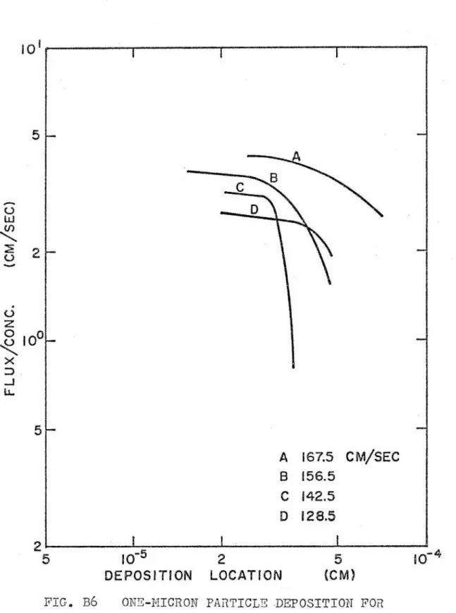
F'igure B6 ^sh:JWS the effect of high .flow rates on the denosi tion of one micron particles when a steady l&"Uinar boundary layer is inrposed al'Jng the wedere. 128.5 crn./sec.

was the lowest velocity used in which at least 3 deposition noints occurred at the wed~e. However, all the deposition points for all the curves are still within one Dicron of the

tip. The inaccuracy of the technique for computing the tra- j ec tori es and the invalidity of' the boundary layer eq"t;_ation at L = 0 make analysis of these se-aara te cu.rve s :meaningless.

However, the general olateau with sharp tail is similar to

lines indicate a ~ig~er ths~rstical deposition valus at L

=

⁰

and then a sharn dip for the :::>eason eDJlai~ed in the last paragr2.ph.

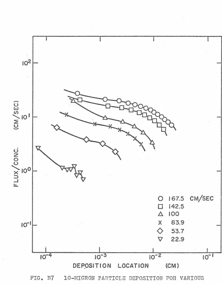
Figure B7 shows the effect of various steady flow rates on the boundary layer denosition of 10 micron ~Jarticles. The general trends of higher deposition f'lu_."C with greater ma7-.imum deposition locations at high V9locities clearly holds. Com- parison of Figure B7 with Figure B3 clearly shm·rn that the shace and locc:.tion of t~e boundary layer depositi0n curve

coincides closely with the sections of the 10 ~icron pot~ntial

• . -? . "' .._, d

deposition curve to the left of 10 - centimeters :rom ~ne we ge tip. This sho";>TS that as the strea.-nJ velocity in ere as es, the boundary layer thiclmess decreases and the inertial forces on the particle increase; therefore, this causes penetration of the bJundary layer and impaction at increasingly greater distances along the wed:·e. The 22.9 cm./sec. curve has an

erratic shape because financial limitations prohibit the excess of C'.):mputer time needed to use a very small time interval in the calculations. The l onger time interval results in a less smooth trajectory and subsequently an erratic deposition pattern.

Friedlander•s Bou.ndary Layer Solution

Friedlander

iu.

· has suggested an analytical solution to

deposition by impaction at a 90° wedge ^;_,rj_ th steady viscous boundary layer. His corrected derivation with some o"I' the author's modirications to account for the uarticle radius is

given in Appendix D.

Friedlander';:; solution assumes that the flow in the boundary layer is rectilinear along the wed§;e -- which is a valid assumption because the value of the perpendicular velocity component from the author's equation is only 10-5 cm./sec. Thus, Friedlander ma_~es the approximation of a steady laminar_ bou..11dary layer ..

However, he then assumes that a p·article entering the

b·::nmdary layer will follow the streamlines along the wedge

and only have an inertial effect perpendicular to the wall.

This will cause the particles to de-oosit on the wall only if they entered the bou~dary layer at a distance within the stopping dist~nce plus the radi~s o~ the particle. The dista.11ce would be evaluated from the potential velocity at the last nosition before entering the boundary layer. The displacement along the wedge WO'.'ld then be dependent on the velocity of the b0Ut.1dary layer and a fraction of the relax- ation time.

Obviously, this solution will predict deposition locations even closer to the wedge tip than the author's results. Since the same relaxation time princinles operate as in the perpen- dicular direction to dailp the particle velocity, one cannot

i~stantly neglect the inertial forces in the ~ direction of a particle entering a boundary layerp

The boundary layer con:rputer 9rogram in this study was nodified to calculate the F /C and deposition location by

s

Fr:Ledl2nder 's solution for all uart icles brea:.·:::ing tb.e ~ = 0

ulane which were within ^{i:;ne . '} the radius '.)f the narticl e from the '.-7edge surface.

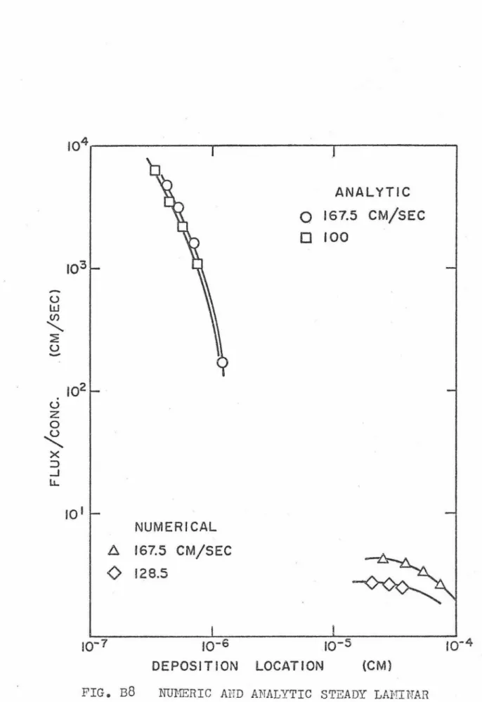
Figure B8 is a comnarison plot of Friedlander's anc..lytic boundary layer solution ^{f J : '} ons micron 9articles at

167.5

and 100 ci11./sec. r-Ji th the author's numerical bou_ridary layer

1 . . . 1 / 7

5

<:>.,..., ' 12A ^r"

I

S·:)_ui:;ion a-c _o • wla u.::; cm. sec. Comparison o.f plots shows clearly that the previous ^argTu.~ents are correct. The analytic plots have all deuosition within 10-7 to

io-

⁶ centi-

~ eters

compared to 10-5 to 10-h centimeters for the author's data. As exuect ed the analytic deposition fluxes uere r:uch higher close~ to the tipo

Figure B9 compares ?riedlander's analytic boundary le.yer solution results for 10 nicron particles at l GO cm./sec. with the author's · _'J.:."Tleri cal boundary l ayer results. In this case the !"er:ions of de9osi ti on overl ap significa.'tltly, however the a•_lthor' s results still shoH deposition further along the wedge. _'-·

The deposition fluxes differ by one to two orders of mag::iitude,.

r-ie apparent increase of flc.cr with distance along the wed!2e for the analytic case is p~zzling at the present time. It is apnarently due to the assw:iption of no inertial ef.fects in the direction ·para1leJ; ·to·:·tha wedge::w.a:ll•:

~x-perimental Procedure

Richard Vincent, an undergraduate strnbnt working for

Professor Friedlander at the California Institute of Technology has collected experimental data for the deposition of 1.099 micron hydrosol particl8s made of Dow Polystyrene Latex in

the lung biflircation model sh:lwn in Figure Cl. A schematic of the exuerimental apparatus is shown in Figure C2. The ca..'71 11.ras desi,c;::ned to simulate a. one second 300 cc breath shown in FigLtre CJ.

Vincent collected, data for 1.0, 1.8, and

2.5

second JOO cc tidal vol1..ll":e breaths by the following procedure. The holding chamber and piston assembly were flushed with aerosols until ths concentration registered about l.5Xl04 particles/cm.3 on a Sinclair-Phoenix Aerosol, Smolce, fu"'1d Dust Photometer.

The ch~~ber was then isolated, the gate lifted, and the cam- driven uiston set in motion. At the end of the stroke the gate 1·rns lowered, and the test section was .flushed gently with a,,-inbient air. This procedure was repeated 30 times to allow sufficient deposition on the glass slides for statis- tically meaningful counts. All singlet particles were counted in an area

.Ol.54

inches wide and one inch long under a micro- scope at

675

magnification.

Analysis of Data

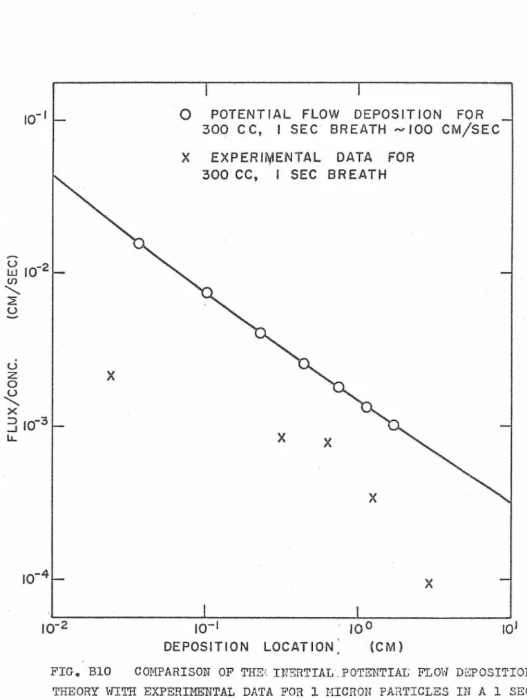
Figures BlO, Bll, and B12 are comuarison nlots of the

aut~or's steady uotential flow data for one micron particles at flow rates of 100,

53.7,

and

41

cm./sec. respectively with Vincent's average exnerimental data for 1.0,

1.8,

and

2.5

second 300 cc breaths. These flow rates correspond to the

average flow rate in the lung model for the respective breaths.

The author's data predict higher deposition rates at all

locations. On each graph the initial experimental data point at .024 centimeters has a deposition flu..ic/concentration value

5

to

8.5

times smaller than the authors predicted potential results. The remaining points are 1 to

5

times smaller than the author's predictions. The two longer breath simulations give better agreement between theoretical and experimental data than the one second breath. Since all boundary layer deposition terminates beyond 10-4

centimete~s,

comparison of experimental data with the one micron steady bou.."'1dary layer reEults of Figure

B4

and B6 is impossible.

The steady potential theory tends to predict deposition values slightly above the experimental results, however the viscous boundary layer theory predicts deposition values far below the experimental results. These relative results for inertial impaction on a wedge generally agree with the results of inertial impaction studies on cylinde.::'s and spheres nre- sented by l"uchs.1

5

In the cylinder and sphere ,cases the experimental data is scattered around the steady potential flow cur'ves, while the viscous flow c1J.rve predicts much lower