A report on the Progress of the Research / Thesis ... - AURA

OPTIMIZATION METHODS IN POWER MARKET AND MACHINE LEARNING ALGORITHMS WITH SUSTAINABLE ENERGIES

PENETERATION

BY

RAMIN FARAJI

A THESIS

SUBMITTED TO THE FACULTY OF ALFRED UNIVERSITY

IN PARTIAL FULFILLMENT OF THE REQUIREMENTS FOR THE DEGREE OF

MASTER OF SCIENCE

IN

MECHANICAL ENGINEERING

ALFRED, NEW YORK

JUNE, 2019

OPTIMIZATION METHODS IN POWER MARKET AND MACHINE LEARNING ALGORITHMS WITH SUSTAINABLE ENERGIES

PENETERATION

BY

RAMIN FARAJI

B.S. IRAN UNIVERSITY OF SCIENCE AND TECHNOLOGY (2009)

SIGNATURE OF AUTHOR

APPROVED BY

EHSAN GHOTBI, ADVISOR

JALAL BAGHDADCHI, ADVISORY COMMITTEE

AMIT MAHA, ADVISORY COMMITTEE

GABRIELLE GAUSTAD, CHAIR, ORAL THESIS DEFENSE

ACCEPTED BY

GABRIELLE G. GAUSTAD, DEAN

KAZUO INAMORI SCHOOL OF ENGINEERING

Alfred University theses are copyright protected and may be used for education or personal research only.

Reproduction or distribution in part or whole is

prohibited without written permission from the author.

Signature page may be viewed at Scholes Library,

New York State College of Ceramics, Alfred University,

Alfred, New York.

ACKNOWLEDGMENTS

I would like to express my gratitude to Dr. Ehsan Ghotbi for his continued guidance throughout the span of this endeavor. To my committee members, Dr. Jalal Baghdadchi and Dr. Wallace Leigh, I give thanks for their assistance. I would like to offer my special thanks to Laura Grove, and Samantha Dannick for the knowledge they contributed. Finally, I would like to thank my parents, my friend and mentor and my best friends Dr. Saeed Ahmadian and Mariah Evans for their moral support. Without them this wouldn’t happen!

TABLE OF CONTENTS

Page

Acknowledgments……….………….iii

Table of Contents..……….iv

List of Tables………..……….v

List of Figures……….vi

ABSTRACT……….……….viii

I. Introduction ... 1

II. published results ... 3

Stackelberg Game Approach on Modeling of Supply Demand Behavior Considering BEV Uncertainty ... 4

Wind Farm Layout Optimization Problem Using Joint Probability Distribution of CVaR Analysis……….…….…………20

Machine Learning Approach in Wind Farm Power Forecasting ... 32

III. Future Work ... 44

IV. References ... 44

LIST OF TABLES

Page

Table II. A. I. Different Characteristics of BEVs ... 12 Table II. A. II. Satisfaction function and generation coefficients . 15 Table II. A. III. Numerical performance evaluation ... 18 Table II. A. IV. Statistical results for generation values in [kw] ... 19 Table II. B. I. Charactristics of the 5 MW wind turbines ... 28 Table II. B. II. Efficiencies of WF under the different scenarios

without CVaR ... 30 Table II. B. III. Efficiencies of WF under the different scenarios

using CVaR ... 31

Table II. C. I. Characteristics of the wind turbine ... 34

Table II. C. II. Annual energy production of the wind turbine ... 34

List of Figures

Page Figure II. A. 1. System model of the retailer company and users ... 7 Figure II. A. 2. Arrival time pdf for BEV owners in rural areas in New York State ... 11 Figure II. A. 3. Departure time pdf for BEV owners in rural areas in New York State ... 11 Figure II. A. 4. Average travelled distance pdf for BEV owners in rural areas in New

York State ... 12 Figure II. A. 5. Required time to fully charge a BEV with respect to distance driven

and car size ... 12 Figure II. A. 6. Stackelberg game theory algorithm ... 14 Figure II. A. 7. Load Profiles for Groups 2 and 3 of Consumers Before and After

Applying Optimization Algorithm ... 16 Figure II. A. 8. Uncertain Load Profile of 50 BEVs Before Applying the Algorithm

without V2G technology ... 16 Figure II. A. 9. Uncertain Load Profile of 50 BEVs After Applying the Algorithm

with V2G technology ... 17 Figure II. A. 10. Load Profiles for Group 1 of Consumers Before and After

Implementing the DR program ... 17 Figure II. A. 11. Aggregated Generation Profiles Before and After Applying

Optimization the Algorithm ... 17 Figure II. A. 12. Conventional and Real-Time Prices Broadcasted by Retailer ... 18 Figure II. B. 1. Jensen's wake effect model ... 23 Figure II. B. 2. Charactristics of the 3 years wind data: (a) wind rose; (b) Weibull

distribution ... 24 Figure II. B. 3. Distribution of: wind speed, direction and joint probability ... 26

Figure II. B. 4. Output power of WF for 25 scenarios without using joint probability

CVaR optimization ... 28

Figure II. B. 5. Wind farm layout without considering the joint probability CVaR ... 29

Figure II. B. 6. Output power of WF for 25 scenarios using joint probability CVaR optimization ... 30

Figure II. B. 7. Wind Farm layout considering the joint ptobability CVaR ... 31

Figure II. C. 1. Power curve of the wind turbine ... 33

Figure II. C. 2. Annual energy production: 21 metre rotor ... 34

Figure II. C. 3.A linear SVM ... 35

Figure II. C. 4. Forecasting flowchart. ... 38

Figure II. C. 5. Cross-validation algorithm ... 40

Figure II. C. 6. Lasso regression scatter result in a 16 by 16 dimension data ... 41

Figure II. C. 7. Cross-validation of the Lasso regression with 19.24% error. ... 41

Figure II. C. 8. SVM scatter result in a 16 by 16 dimension data... 42

Figure II. C. 9. Cross-validation of the SVM with 28.98% error ... 42

ABSTRACT

The targeted goal of the renewable energies in the recent years has received more attention due to the high volume of the world pollution, greenhouse gases and global warming. Moreover, the process of the control and monitoring of the renewable energies has always been an issue and since the climate change might not have a recognized patterns in different locations, researchers and scientists look for optimizing the better use of the sustainable energies and increase the efficiency. One of the problems with the renewable energies such as solar or wind power is that they cannot be trustworthy and in power planning context, having a forecast about the future power need for the consumers is critically essential. By mathematical modelling, researchers try to formulate these environmental impacts to be able to forecast them and plan on a long-term usage of sustainable energies. This thesis along with the published works mentioned in the following talks about control and monitoring the power market with different approaches.

At first, I looked at the households with battery electric vehicles (BEVs) penetration in New York State and how the increasing number of the BEVs can affect on the power market and how a smart grid can shave the high demand picks of hours. By this look, we maintained the electricity usage of the consumer alongside with respect to the least pressure on the grid. The proposed algorithm can benefit both the consumer and the electricity provider in terms of pricing and pressure. Moreover, the next argument is about the optimized locations wind turbines in a wind farm. By the proposed algorithm and micrositing, we can guarantee the maximum power generation of the wind farm and address the forecasting issue. In the meantime, machine learning algorithms can benefit us with the forecasting of the wind power generation for the future. Here we discuss about how the machine learning and artificial intelligence can improve our understanding of the power generation forecast for the sustainable energies.

I. INTRODUCTION

In recent years, number of electric vehicles (EVs) is increasing rapidly. The EV batteries may be programmed to have two-way communication with power grid. With the development of charging facilities, it is possible to send/receive power from electric vehicles. This feature could be utilized to dispatch energy back to the grid when there is an outage. The second hand batteries from old electric vehicles could also be employed to smooth the intermittent renewable energy generation.

By installing renewable energy units such as wind, solar, biomass in distribution network adjacent to consumers, small scale power systems can be formed called microgrid. The aim of this study is to examine the correlation between electric vehicles and renewable energy generation in a microgrid.

Generation and load are both exist in microgrids and this could provide many opportunities for grid operators. For instance, during power outage conditions, islands can be formed to meet the load with minimum amount of load shedding. The main drawback of renewable energy is the intermittent nature of it. The most suggested viable practice is energy storage system. The interaction of electric vehicles and renewable energy could be a topic that has to be addressed because they will help to build the microgrids.

In the next sections, first, day ahead planning approach is considered to manage power grid, renewable energy generation and electric vehicles. We present an algorithm to smooth the impact of electric vehicle charging on power grid. In addition, the possibility of using the extra energy stored in electric vehicles battery is studied. After we propose the possible actions for managing electric vehicle charging challenge for current state of the grid operation, then the trend of electric vehicle purchases is investigated and the possible correlation between the number of electric vehicles being purchased in each year and renewable energy expansion plans is examined.

After possible corrective actions are determined for microgrid operation, the real time operation of the system needs to be studied. For this purpose, all the components of

microgrid including extra renewable energy units, electric vehicles and transmission lines are simulated in real time simulator.

This study can be regarded as a comprehensive study of microgrid which could be used for future planning policies and energy management systems.

II. PUBLISHED RESULTS

The following studies have been carried out in this thesis study and their results have been published/submitted in various papers and poster:

A) B. Azimian, R. F. Fijani, E. Ghotbi and X. Wang, "Stackelberg Game Approach on Modeling of Supply Demand Behavior Considering BEV Uncertainty,"

2018 IEEE International Conference on Probabilistic Methods Applied to Power Systems (PMAPS), Boise, ID, 2018, pp. 1-6.

B) R. Farajifijani, Ahmadian, S., Ebrahimi, S. and Ghotbi, E., 2019, January.

Wind Farm Layout Optimization Problem Using Joint Probability Distribution of CVaR Analysis. In 2019 IEEE 9th Annual Computing and Communication Workshop and Conference (CCWC) (pp. 0007-0012). IEEE.

C) Fijani, R.F., Azimian, B. and Ghotbi, E., 2019. Game Theory Approach on Modeling of Residential Electricity Market by Considering the Uncertainty due to the Battery Electric Vehicles (BEVs). arXiv preprint arXiv:1902.05028.

D) Ahmadian, S. and Farajifijani, R., 2019. A New Method To Find The Nash Equilibrium Point in Financial Transmission Rights Bidding Problem. arXiv preprint arXiv:1902.09329.

E) Farajifijani, R. and Ghotbi, E., 2018. Wind Farm Micrositting Optimization by Stackelberg Game Theory Model. Scholes Library.

F) Farajifijani, R., Ahmadian, S., Ebrahimi, S. and Ghotbi, E., 2018. Application of CVaR (Conditional Value at Risk) Analysis In Wind Farm Layout Optimization. Scholes Library.

The contents of these published manuscripts will be found in the following sections of this chapter.

Stackelberg Game Approach on Modeling of Supply Demand Behavior Considering BEV Uncertainty

Abstract

Based on advanced metering infrastructure (AMI), one can use big data to provide demand-response (DR) solutions. There is a need to develop optimized cost structures for consumers. In this paper, Stackelberg game approaches are utilized, and residential loads are considered including battery electric vehicles (BEVs) equipped with BEV communication controllers and vehicle-to-grid (V2G) technologies. Efficient and effective optimized algorithms are developed for users (followers) based on time dependent pricing schemes. In the “games,” besides the followers, other participant is an electricity retailer company (leader), with a two-way bilateral communication procedure accepted and established by all participants. The user side of the games is related to the demand side management (DSM). Real-time pricing (RTP) from time-of-use (TOU) companies is used to achieve better results. Monte Carlo simulations (MCS) represent uncertain behaviors of BEV drivers. Results indicate that customers’ demands can be met while reaching the best efficiency.

I. Introduction

In a traditional power grid, proper metering may decrease demand response (DR) non-scheduled loads slightly. In a smart grid, several advanced techniques can be integrated, including advanced metering infrastructure, energy management systems, distributed energy systems, intelligent electronic devices, internet of things (IoTs), and battery electric vehicles (BEVs) [1]. When a smart metering infrastructure is combined with DR programs, efficiency can be improved [2]. Two types of DR have been discussed previously: 1. The retailer has all the power to directly control consumers’

usage which decreases the satisfaction of the users; and 2. The retailer reshapes DR programs through dynamic pricing such as critical pricing and real time pricing (RTP) [3]. The second type is preferred in this study.

Modern energy managements via smart grids may take advantages of following technology developments: bi-directional energy flows, price-responsive loads, intelligent electronic devices (IEDs), and phasor measurement units (PMUs). Thus, sophisticated

smart metering facilities and advanced two-ways communication technologies enable more flexible energy generations, deliveries and consumptions [4-7]. In a self-scheduling model simulation, consumers can participate “day-ahead” energy markets in order to minimize costs and/or maximize profits [8]. Price uncertainty was studied for generation company as a leader in game theory framework [9-10]. Recently, game theories are being considered in DR solutions and load peak shavings. In references [11-12], a Stackelberg game approach was used to deal with DR scheduling under load uncertainty based on real-time pricing in a power grid. In references [13-14], similar approaches were used to stimulate a power company and its customers to “play the game” in order to maximize their benefits and to eventually flatten aggregated load curves. With bi-level hybrid multi-objective evolutionary algorithms, utility companies’ profits may be optimized [15]. Additionally, various approaches have been developed to find the clearing price in retail electricity markets with high penetrations of renewable energies. Based on a time- of-use (TOU) pricing structure, providers or retailers can charge a calculable fee for the fixed price depending on an amount of consumption during a specific time interval [16- 17]. Commonly, electric vehicles are connected to grids to receive energy, and limited savings can be achieved when charging schedules are adjusted to avoid peak load periods [18]. In a case study, benefits of the coordinated EV charging strategy were considered in terms of energy cost savings and peak-to average ratio reductions [19]. An autonomous energy management system was used to allow residential users selling energy back to the utility company by discharging the PEV’s battery [20]. An optimization approach was suggested to provide an optimal charging strategy for the EVs to proactively control their charging speed to minimize the cost of charging [21]. An online electric vehicle scheme was considered to provide electric power to the vehicle wirelessly by a smart grid [22].

With a power payment function, the smart grid can maximize the social welfare of the online electric vehicle’s needs.

Using Stackelberg game theory approach, performance can be substantially improved with a demand response program [3]. To our best knowledge, there is no literature in public domain to systematically consider electric vehicle owner’s driving behaviors via the game theory. In this study, a mixed integer nonlinear programming scheme is considered to achieve benefits for both “energy providers” and “consumers.”

A new approach is considered here to flatten peak loads by scheduling times slots home appliances and BEVs which can be charged and discharged via two-way technologies by combing grid-to-vehicle (G2V) and vehicle-to-grid (V2G) connectivity. By using V2G technologies, retailers can buy energy from consumers if such practices are mutually beneficial. Thus, the following sections will study advanced two-way communication links and BEVs charging/discharging schedules to maximum utility companies’ profits via peak-shaving, and to satisfy consumers by elevating their roles to participants and to minimizing costs. Using a price-based model to guarantee an efficient algorithm between an electricity retailer and users owning BEVs with the aim of balancing the load.

Main contributions of this paper include following key points:

 Using a price-based model to develop an efficient algorithm between retailers and users (with BEVs), and aiming for balanced supply-load by shaving peaks;

 Generating optimized results for both retailers and users with an iterative algorithm, and finding Stackelberg equilibrium (SE) to achieve optimal loads for both parties;

 Formulating 1-N leader-follower Stackelberg relationship between one retailer and N users; and adopting the RTP function of the retailer and the utility function of N users; and

 Handling uncertainty of different driving habits of BEV owners by MCS.

Specifically, the rest of the paper is organized as follows. Section II discusses the system model and formulates the Stackelberg game theory. In Section III, we use data to generate load profiles of BEVs. Some key aspects of Stackelberg game theory and the logic are presented in Section IV. Results are provided in Section IV, and conclusions are drawn in Section V.

II. SYSTEM MODEL

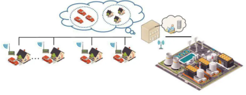
In Fig. II. A. 1, a model is created for one utility company and N users with BEVs. These users will adjust their electricity usages by using advanced metering infrastructure and heterogeneous communication technologies, with the ultimate goals to reduce overall costs. The utility company (retailer) can provide hourly price structures to these users to encourage peak shaving and ultimately to maximize profits.

Advanced communication technologies enable the cloud computing environment and real time sensing/controlling including IoTs [23]. In this environment, an entity represents an electric load (consumer) or a prosumer such as a BEV. In the cloud environment, the real-time access to each entity is guaranteed. The system operator can categorize users into different groups. As shown in Fig. II. A. 1. all prosumers can be placed in one group, and other conventional loads in other. By utilizing instantaneous two-way communication links, real-time electricity prices will be broadcasted, conventional users’ consumption behaviors will be adjusted, and BEVs charging/discharging schedules can be changed. To maintain system stabilities and guarantee maximum profits, the retailer can impose load curtailment during peak hours.

Fig. II. A. 1. System model of the retailer company and users.

A. Retailer Company Model

In this model, the cost function for the retailer is labelled as 𝐶_𝑡(𝑔_𝑡), and depends on the amount of electricity provided (g_t) during an interval t ; where t T T , T that is a strictly convex and monotonically increasing function.

 

t ₂^t t² t t t t

a g g

C g  b c (1)

Where a b_t, _tandc_tare the generating coefficients. During different time intervals, each coefficient has a different value.

Taking a differential operation against (1), one obtains the marginal cost function Ct:

( )

t t t t t

C g a g b (2)

which is the cost to produce one more unit of electricity. Such marginal cost must be lower than the actual cost in order to guarantee profits for the retailer company. So, market price equation can be defined:

   

^{( )}

t gt t gt t atgt t

P tC  b , t1 (3)

whereP_t is price at each time slot and_tis a time-wise profit coefficient. In reference [15], a similar profit coefficient was introduced, minimized and validated. In this paper, there are 24 time intervals (slots), corresponding to 24 prices in a day. The retailer provides electricity and its price to the consumers who will decide how much to use in each time interval. Thus, a user can move his/her electricity usages to off-peak intervals to minimize the total costs. The retailer wants the most profit and the least aggregated peak load in order to avoid expensive backup generators. Flattening the demand load should be two-ways as a user has critical needs for electricity. To determine the optimal generation vector, one should minimize variations in generation, and match supply with demand. Therefore, the retailer problem can be formulated as follows:

 

²

min _RC( _t) _t

t T

U g g g

   (4)



^max



s.t. L_t g_t min g_t^,L_t (5)

_,

1 N

t n t

n

L l

  (6)

¹ _{, ,}

1 N

t i t n t

i

L l l i n



    (7)

Where U_RCis the utility function of the retailer company and g is an average power generation during a day. _Lt is the summation of electricity demands of all N users during the time interval t. gt^ is the maximum capacity of the retailer company’s generation at the interval t, Lt^max is the overall upper bound of the total power demands for slot t.l_{n t,} is the power consumed by user n in the interval t One must notice that the above-mentioned function is different from profit maximization. In (4), minimizing utility function may

lead to maximized profits. In (5), the generation should always meet the total demand of all users, and be lower than the smallest threshold for generation capacity and upper load ranges. In (6) and (7),L_t can be obtained by asynchronous user’s adjustment of consumption, reflecting the human nature that no two users will react to real-time pricing schemes due to different needs. In (7), a user adjusts his/her usage, while others don’t. In such non-simultaneous framework, no two users will negate their effects by increasing and decreasing their demands at the same time.

B. User Model

Each user has its own utility function, shown in (8). According to what has been explained in Section II, with the application of IoTs, the user can be an entity representing an electric load (consumer) as the first term, or a prosumer such as a BEV as the second term. Function _{n t,} (x_{n t,} ) models the satisfaction of the electricity consumers;

in which x_{n t,} is the general power consumption variable, l_{n t,} being the residential demand and s_{n t,} being BEV demand. The third term is the total amount of money to be paid by the consumers, which leads to less satisfaction as represented by a negative sign.

With this, the demand side problem is formulated as follows:

^{   }

    

24 , , 1

24 24

, , , ,

1 1

, arg max ,

. . .

n n n t n t n t

BEV BEV

n t n t n t t n t n t n

t t

l s U l s l

s P P g l s P







 

  

 

  (8)

 

²

, , , , , , , 0 , 0

2

n

n t xn t n txn t  xn t n t n t

       (9)

, , ,

s.t. l_{n t}^ l_{n t} l_{n t}^ (10)

24

1 n t, n t

l L

 

 (11)

24 1 ,

req

n t n

t

s T

 

 (12)

24 max

1 n t, n t

s T

 

 (13)

, dep n

SOCn T BC (14)

where _{n t,} is the preference parameter with indices n (user) and t (time), _nis a predetermined constant integer, L_nis the total daily energy usage,s_{n t,}  { 1, 0,1} is a discrete variable which is multiplied by rated battery power P^BEV of electric vehicles and indicates BEV charging {1}, discharging {-1} status. If it is charging, it will have a positive effect on satisfaction of the utility function, and if it is discharging, it has a negative effect. Although discharging has a negative effect on satisfaction, it is losing the power obtained in the past charging periods. However, by selling discharged electricity, it has positive effect on the third term of utility function. T_n^reqis the required time to fully charge the BEV, T_n^maxis the maximum number of hours that the battery is interacting actively with the network, ,

, dep n T

SOC shows the BEV state of charge, and BC_n is the battery capacity, T^depis the vehicle’s departure time from the house. (9) Denotes the satisfaction function_{n t,} (x_{n t,} )of the user n by consuming l_{n t,} amount of electricity. (10) provides the upper and lower boundaries for electricity demand of n^th user n for interval t.

(11) expresses the temporally-coupled constraint which wouldn’t reduce the total daily consumption of the user n, so we can apply load shedding only in terms of pick shaving and load shifting. (12) states the cumulative charging time in order to fully charge the BEV before leaving one’s residence. (13) limits the maximum number of hours for a BEV connected to the grid system, either in G2V or V2G mode. Therefore, by limiting the hours that the battery is being charged or discharged, we reduce the detrimental effect of constant battery usage. In (14) the sequence of charging/discharging should be in a way that by the time that the BEV owner decides to leaves the house, the SOC should be 100%.

In the Stackelberg equilibrium context and the hierarchical process, our aim is to maximize the leader’s (retailer) utility function by having the data of the follower’s (user) rational reaction set (RRS). The existence of the Stackelberg equilibrium has been discussed and shown in [4]. In addition, the model in (8) is formulated as a mixed integer nonlinear programming problem, and can be solved via MATLAB-GAMS interface.

III. BEV LOAD PROFILE

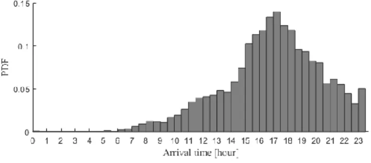
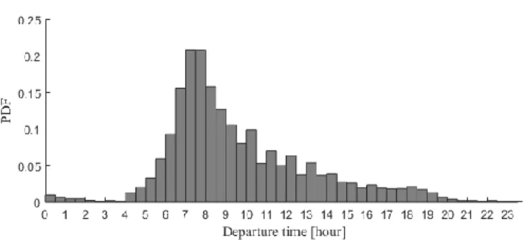
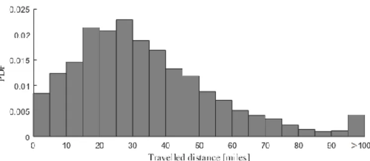
To model BEV load profiles, data from National Household Travel Survey (NHTS) for rural New York State were utilized to estimate average driving mileages and optimize battery usages. The SOC of the vehicles upon their home arrival time is of crucial importance [24]. Table II. A. I. shows the data according to different types of cars and different characteristics. Also, in Figs. 2-4, probability distribution functions (PDFs) for driving behavior, including arrival time, departure time, and traveled distance in rural areas in New York state has been drawn from NHTS data. The reason why we chose rural areas in New York State is that Alfred University is located in rural areas.

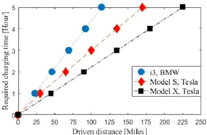
Moreover, configuring the time of fully charged BEV depends on the distance it travels daily, and we assume that BEV is a constant power prosumer. From Fig. II. A. 5. we obtain the required charging time based on daily driven distance [25-26].

Fig. II. A. 2. Arrival time pdf for bev owners in rural areas in new york state.

Fig. II. A. 3. Departure time pdf for bev owners in rural areas in new york state.

Fig. II. A. 4. Average travelled distance pdf for bev owners in rural areas in new york state.

Fig. II. A. 5. Required time to fully charge a bev with respect to distance driven and car size.

Table II. A. I. Different Characteristics Of BEVs

Vehicle Type

Commercial model

Expected Market Share [%]

Energy [kW-hr]

Rated Battery

Power [kW]

Single Charge Drive- Range [mile]

Compact

sedan i3, BMW 51.48 33 7 114

Mid-size sedan

Model S,

Tesla 10.35 75 11.5 259

Mid-size SUV

Model X,

Tesla 38.17 100 17.2 295

IV. STACKELBERG GAME THEORY ALGORITHM

In Fig. II. A. 6. iterative DR algorithm is illustrated via a flow chart. At the beginning of the computation, the retailer broadcasts hourly price one hour ahead.

According to (3), marginal cost function is calculated by power generation requirement and initial price broadcasted. As the relationship between the price equation and power is linear, the algorithm uses the generation value. Final prices can be found once the total power generation value is known. Afterwards, Monte Carlo simulation emulates driving behaviors of BEV owners.

Users respond to the prices broadcasted, and shift their usages to non-peak time slots. BEV discharging features can help the retailer company to offset some loads during peak hours. The peak-shaving and the demand aggregation can be accomplished continuously instead.

Fig. II. A. 6. Stackelberg game theory algorithm.

V. SIMULATION AND RESULTS

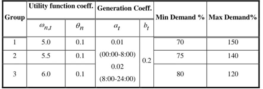
Residential consumers are divided into three groups as tabulated in Table II A. II.

Group 1 corresponds to utility function coefficient_{n t,} of 5.0, with 50 BEVs. Groups 2 and 3 do not have BEVs, but have different utility coefficients. The minimum and the maximum values refer to the lower and upper bounds of the targeted power demands.

For example, Group 1 consumption varies between 70% and 150% of its nominal load.

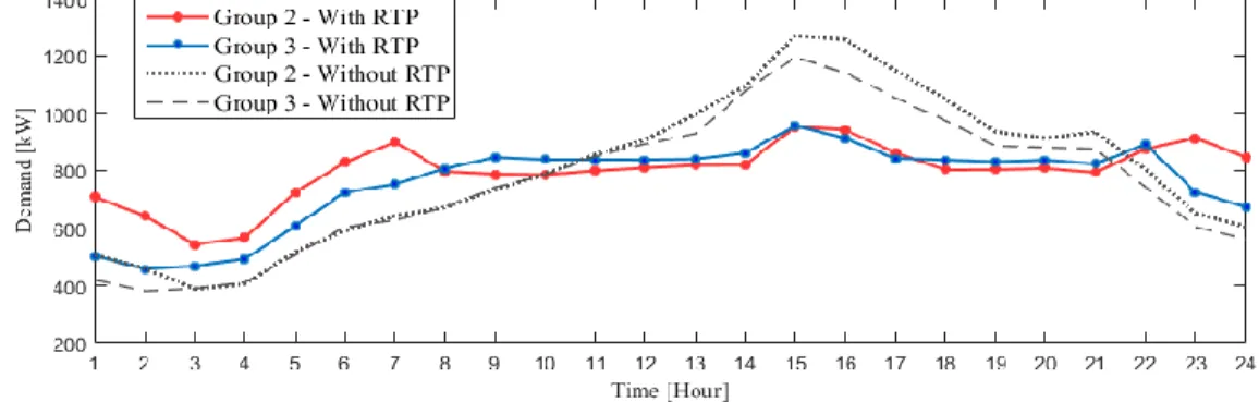
The price coefficient is kept constant, i.e., t1.2. In Fig. II. A. 7, load profiles are shown for Group 2 and 3; and benefits from the game theory applications can be visualized by examining a profile with or without the algorithm. In general, the load profiles are flattened due to users’ participations. In comparison with Group 2, Group 3 shows less eagerness to participate as it has larger _{n t,} . For group 1, as illustrated in Table II. A. II, managing the vehicle’s V2G or G2V status is of great importance.

Table II. A. II. Satisfaction Function And Generation Coefficients

Group

Utility function coeff. Generation Coeff.

Min Demand % Max Demand%

,

n t n _{at bt}

1 5.0 0.1 0.01

(00:00-8:00) 0.02 (8:00-24:00)

0.2

70 150

2 5.5 0.1 75 140

3 6.0 0.1 80 120

If a large number of BEV owners begin to charge their vehicles immediately returning home, the sudden power load may be undesirable. By applying the algorithm in Fig. II. A. 6, the uncertainty related to random behaviors of BEV owners can be managed by optimizing charging and discharging activities. In Fig. II. A. 8, wide bands of load profile for BEVs are shown for each time slot in a day. Without game theory applications, the users’ peak load can coincide with that of the BEV charging peaks. In Fig. II. A. 9, modified BEV load profile is obtained after applying the algorithm. The negative values represent the V2G feature of the BEVs, or discharging. After coming back to home (between 17:00 or so and midnight), most vehicles are either sending back power to the grid or in standing by mode. The charging period mainly happens between

1:00 and 6:00. Comparing the time interval between 14:00 to 16:00 in Fig. II. A. 7 and Fig. II. A. 10, more peak shaving has been achieved for

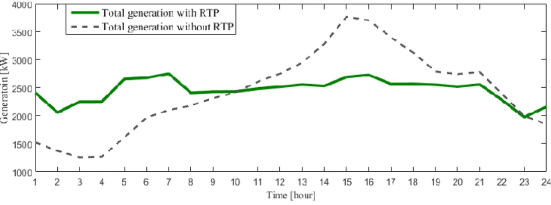
Group 1 due to the presence of V2G technology. Fig. II. A. 11 shows the total generation over 24 hours for users’ aggregated demand with and without implementing the DR program. The expected value at each hour is used to obtain the profiles in Fig. II.

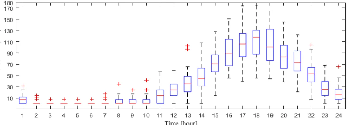
A. 10 and Fig. II. A. 11. From Table II. A. IV, the standard deviation shows that more fluctuations will happen mainly from 22:00 to 24:00 and 1:00 to 5:00. Therefore, the power system operator should consider more spinning reserve after midnight; this will cause an increase in power system operation cost. Finally, the real-time prices over 24 hours that has been derived from the algorithm is compared with the conventional price in Fig. II. A. 12. The performance of the algorithm is evaluated by two scenarios (with and without RTP and V2G) from various aspects.

Fig. II. A. 7. Load profiles for groups 2 and 3 of consumers before and after applying optimization algorithm.

Fig. II. A. 8. Uncertain load profile of 50 bevs before applying the algorithm without v2g technology.

Fig. II. A. 9. Uncertain load profile of 50 bevs after applying the algorithm with v2g technology.

Fig. II. A. 10. Load profiles for group 1 of consumers before and after implementing the dr program.

Fig. II. A. 11. Aggregated generation profiles before and after applying optimization the algorithm.

Fig. II. A. 12. Conventional and real-time prices broadcasted by retailer.

The numerical results are shown in Table II. A. III. The peak demand is significantly decreased by almost 1 MW. Total energy usage has not been changed, which proves that the retailer cannot reduce the whole amount of energy that a user expects to consume per day. This reality is shown in (11). Using algorithm in Fig. II. A.

6, the total user payments decreased about 16%, which demonstrates the efficiency of game theory application. Additionally, the generation costs of both scenarios can be less than the total payments, i.e., making profits for the retailer.

Table II. A. III. Numerical Performance Evaluation

Scenario Peak demand [kw]

Total Energy Usage [kwh]

Total Payments [$]

Generation Cost [$]

Without RTP and Without

V2G

3841 59092 36135 15115

RTP and V2G 2755 59092 30244 12661

Table II. A. IV. Statistical Results For Generation Values In [Kw]

Time [hour] 1 2 3 4 5 15 16 17

gtExpected value 2412 2060 2255 2256 2659 2694 2732 2571

gtStandard deviation 66 76 26 28 42 29 49 12

Time [hour] 18 19 20 21 22 23 24

gtExpected value 2573 2556 2524 2561 2283 1976 2163

gtStandard deviation 14 14 8 16 130 66 197

CONCLUSION

Using game theory algorithm, one can reduce costs to consumers and potentially reshape generating profiles. In this paper, a model included one retailer and N users (with some of them owning BEVs). In particular, an optimized approach can shave peaks with DR managements. The game theory and Stackelberg equilibrium have been utilized to illustrate an algorithm for three different user groups. By comparing the results with and without DR managements, the efficiency of the algorithm can be shown. Using MCS in MATLAB-GAMS, the stochastic behavior of BEVs are simulated. According to the statistical analysis, such algorithm based on the game theory can reduce the peak loads.

We are currently investigating possibilities to include more leaders and followers as well as incorporating solar and wind energy.

Wind Farm Layout Optimization Problem Using Joint Probability Distribution of CVaR Analysis

Abstract

This study proposes the optimal layout of an offshore wind farm (WF) allocation for a number (N) of wind turbines (WTs) in a 2 km × 2 km fixed area. The paper aims to maximize expected WF power output and efficiency, considering the joint probability distribution of wind speed and direction. In fact, the effects of both stochastic variables (wind speed and direction) are considered to find optimal WF layout. Unlike most previous studies, using the coordinate model (CM) allows the WTs to be located on any available spot in the WF but not only at the center of the grids. Thus, by applying joint probability

distribution to the WF expected power output; a new multivariant conditional value-at- risk model is being presented to find the best possible layout under the worst-case scenarios for both wind speeds and directions. Indeed, the presented optimization model obtains the optimal WF locations, while it guarantees the robustness of the WF layout with certain confidence level (1 – α). Finally, a case study with actual manufacturer data for the same WTs with realistic wind profile data are performed under the scope of this research to show the robustness of presented model.

I. INTRODUCTION

As a worldwide concern about reducing the greenhouse gas emissions and growing price of oil, scientists and politicians have paid more attention to renewable energy resources especially wind energy. Wind energy is the most profitable source of renewable energies with the capacity of being located all over the world. Huge growth in wind energy to anticipate sector of electricity for a sustainable future has led the scientist and researchers to constantly, look for the optimal methods to harness power output in the most efficient way. Thus the properties and behaviors of the wake effects on turbines and WFs, which reduce and disturb the wind (velocity deficit) in downwind flows behind the rotors, has become an important topic to discuss.

Many approaches have been studied due to increase the profit and minimize the investment costs and to find an optimal layout for WTs micrositing. Marden, Ruben and

Pao [27] has done a complete survey to demonstrate the application of game theories in wind farm optimization which resulted to the fact that distributed algorithm could benefit for wind farms economic aspects. Moreover, another approach has been proposed by a model-free control strategy machine learning algorithm by studying a set of optimal induction factors under controlled WF wind conditions and achieved 25% more efficiency compared to greedy algorithms [28]. Numerous wake effect models and optimal layout approaches have been studied to maximize the efficiency at minimum wind farm costs and maximum power harness [29]-[38]. Gao proposed a newly developed two-dimensional wake model where, he analytically used Gaussian function for computing Jensens wake model [39]. In [40], researchers suggested discrete optimal WTs locations by employing multi-objective evolutionary algorithm (MOEA/D) to provide flexible options to calculate desirable efficiency with selected WT numbers. A number of researchers such as [41] worked on mathematical aspects of wind farm optimization using fuzzy genetic models to enhance the speed of calculation and computation cost.

To organize the rest of this work, the authors introduced the methodology and the mathematical modelling in section II, proposed approach and the application of the algorithm and its optimized results in section III. Finally, section IV draws the conclusion for the presented paper.

II. MATHEMATICAL MODELLING

In this section, the algorithm and mathematical modelling of WF will be addressed. First, a comprehensive model is set up. A WF consisting of WTs which has been defined by the set of N =: {1, 2, …, n} where the characteristics of the WTs are mentioned in Table II. B. I. Also, the Weibull distribution with the scale parameter λ and the shape parameter k is assumed for the wind speed v. Meanwhile, the Normal distribution is considered for the wind direction θ. Thus, the wind speed and direction are formulated as:

𝑓_𝑣(𝑣, λ, 𝑘) =𝑘 𝜆(𝑣

𝜆)

𝑘−1

𝑒𝑥𝑝 (− (𝑣 𝜆)

𝑘

) (1)

𝑓_𝜃(𝜃, 𝜇, 𝜎) = 1

𝜎√2𝜋𝑒𝑥𝑝 (−(𝜃 − 𝜇)² 2𝜎² )

Considering (1) and distinctive wind speed and direction as two independent stochastic variables, the joint probability distribution is as follows;

𝑓_(𝑣,𝜃)(𝑣, 𝜃, λ, 𝑘, 𝜇, 𝜎) = 𝑓_𝑣 (𝑣, 𝜆, 𝑘) × 𝑓_𝜃(𝜃, 𝜇, 𝜎) (2)

Since most offshore WFs are allocated rectilinear grids shape, a 2 km × 2 km rectangle, tilted and rotated plane ground is defined.

A. Wake Effect Model

Although the Katic wake model [42] has been widely used by researchers, the Jensens model [43], [44] is still the most accepted and fastest model to find the wind velocity decay. The wake decay generated by the turbine i located at point 𝑇_𝑖 is being modeled as a conic shape. According to Fig. II. B. 1. the wake effect of turbines i on turbine

𝑗 = 1, 2, … , 𝑛, 𝑖 ≠ 𝑗 with the angle 𝛽_𝑖,𝑗,which is the axis to axis angel between WTs and point A, and the wind expansion k can be obtained with the following equation:

𝜓_𝑖,𝑗 = 𝑐𝑜𝑠⁻¹ [

((𝑥_𝑖 − 𝑥_𝑗) cos 𝜃 + (𝑦_𝑗 − 𝑦_𝑖) sin 𝜃 +𝑅 𝑘)

√((𝑥_𝑗 − 𝑥_𝑖 + (𝑅

𝑘) cos 𝜃)²+ (𝑦_𝑗− 𝑦_𝑖 + (𝑅

𝑘) sin 𝜃)²]

(3)

Where 𝜓_𝑖,𝑗 is the wake effect between WTs, (𝑥_𝑖 − 𝑥_𝑗) and (𝑦_𝑗− 𝑦_𝑖) are the coordinates of the WT i and j and R is the WT radius. As Kusiak and Song [45] showed in their work, only the scale parameter of the Weibull distribution is being impacted. In this case, The velocity deficit at j^th turbine is defined as:

𝑣_𝑗^𝑑𝑒𝑓 = √ ∑ [ 1 − √1 − 𝐶𝑇

(1 + (𝑘 𝑅)𝑑^𝑖,𝑗)

2]

2 𝑛

𝑖=1,𝑖≠𝑗,𝜓𝑖,𝑗<arctan (𝑘)

(4)

While 𝐶_𝑇 is the thrust coefficient and di,j is the projected distance between two turbines and direction𝜃.

B. Turbine Power Output Model

The expected power output yield of all the WTs are identical and follow the equation (5):

𝑃(𝑣) = {

0 𝑣_𝑖 > 𝑣_𝑐𝑜 , 𝑣_𝑖 < 𝑣_𝑐𝑖 𝑒^𝑣𝑖

𝑎 + 𝑏^𝑣𝑖 𝑣_𝑐𝑖 ≤ 𝑣_𝑖 < 𝑣_𝑟 𝑃_𝑚𝑎𝑥 𝑣_𝑟 ≤ 𝑣_𝑖 < 𝑣_𝑐𝑜

(5)

Where P is the power output, Pmax is the rated power, v is the wind velocity, vci and vco

are the cut-in and cut-out wind speed, a and b are the logistic function parameters.

Fig. II. B. 1. Jensen’s wake effect model.

C. Coordinated Model (CM)

The coordinate model (CM) [46] has been used due to the flexibility of the ATs allocation with higher accuracy to locate the optimum benchmarks. Therefore, according to the following formulations any point on our farm (𝑥_𝑗− 𝑥_𝑖) is a potential spot for the WTs.

max ∑ 𝐸(𝑃_𝑖)

𝑁

𝑖=1

= ∑ ∑ 𝑓_(𝑣,𝜃)^𝑠 𝑃_𝑖^𝑠

𝑆∈(𝑣,𝜃) 𝑁

𝑖=1

(6) 𝑠. 𝑡. 𝑥_𝑙+ 𝑅_𝑖 ≤ 𝑥_𝑢 − 𝑅 (7)

𝑦_𝑙+ 𝑅 ≤ 𝑦_𝑖 ≤ 𝑦_𝑢 − 𝑅 (8)

(𝑥_𝑖 − 𝑥_𝑗)²+ (𝑦_𝑖 − 𝑦_𝑗)² ≥ 64𝑅², ∀𝑖, 𝑗 ≔ {𝑖 ≠ 𝑗} (9)

𝑖, 𝑗 = 1, 2, … , 𝑁 (10)

Where s is corresponding scenario for the pair of (𝑣; 𝜃) and 𝑓_(𝑣,𝜃)^𝑠 is the scenario probability, u and l indexes present the upper and lower bounds of the wind farm and 𝐸(𝑃_𝑖) is the expected value of power generation, respectively. Equation (9) is the distance constraint, same as previous studies, which is the safety factor to assure that the minimum distance between two WTs is more than four times WT radius (R).

Fig. II. B. 2. Characteristic of the 3 years wind data: (a) wind rose, (b) Weibull distribution.

D. Conditional Value at Risk (CVaR)

Due to the uncertainties of the wind direction and speed, the market loss ranges from 30% to 50% has always been guaranteed. Even with the best prediction tools, the wind farm owners have been suffered from this uncertainty. The application of the value at risk (VaR) and CVaR including their advantages and disadvantages has been discussed in [47]- [52]. Although VaR suffers from lack of sub-additivity and convexity, using CVaR allows applying it to the linear programming optimization algorithms. Therefore, finding the expected value of the worst cases scenarios (1 − 𝛼) of profits is being calculated by a more conservative risk measurement method. Additionally, with the coherence of the CVaR method, the risk measurement has preserved the convexity of the robust optimization (RO) counterpart to the optimization problem with the uncertain data, which is also tractable. CVaR can be used as either an objective function, constraint or both. Here, we add CVaR constraints to the coordinate model to deal with the wind uncertainties while maximizing the value of wind farm energy production. Thus, given the following equation with 𝛼 being the confidence level as a given parameter:

𝛼 ∈ (0,1) , 𝐶𝑉𝑎𝑅_𝛼(𝑝𝑟𝑜𝑓𝑖𝑡) = 𝐸[𝑝𝑟𝑜𝑓𝑖𝑡 | 𝑝𝑟𝑜𝑓𝑖𝑡 ≤ 𝐶𝑉𝑎𝑅_𝛼] (11) Since the wind parameters (speed and direction) are uncertain, the CVaR was applied to the both velocity and direction equations. Considering 𝑔(𝑥; 𝜃; 𝑣) as profit function for WF, which depends on decision variables (x) and uncertain variables (𝜃; 𝑣), the CVaR formulation for the uncertain wind direction is determined as:

𝑓𝑜𝑟 𝑢𝑛𝑐𝑒𝑟𝑡𝑎𝑖𝑛 𝑣𝑎𝑙𝑢𝑒𝑠 𝑜𝑓 𝜃 ∈ {𝜃₁, 𝜃₂, … , 𝜃_𝐾𝑠} 𝐹_𝛼(𝑥, ξ) =

ξ − 1

1 − 𝛼× ∑ (∑[𝜉 − 𝑔(𝑥, 𝜃, 𝑣)] × 𝑓_𝑣,𝜃(𝑣, 𝜃, 𝜆, 𝑘, 𝜇, 𝜎)

𝐾_𝑠

𝑖=1

) × 𝑝(𝑠)

𝑠∈𝑆

(12)

Where 𝐹_𝛼 (𝑥, 𝜉) is the CVaR function approximation for uncertain parameters, ξ is the largest amount such that P(u) is equal to its minimum value, α is the confidence level, Ks

is the number of samples with respect to the scenario s and p(s) is the probability of each scenario.

III. OPTIMIZATION MODELLING AND RESULTS

Applying the CVaR model directly to the WF objective function brings the fact that minimum energy output of the WF is always higher with confidence level (1 − 𝛼). It is assumed a 5 by 5 scenario matrices to find the probability of each. From the WF owner stand view, it was assumed, 80% power output of the WF should be satisfied by the optimized allocation of WTs. Therefor considering 1 − 𝛼 = 0.95 , for 95% of possible scenarios, the achieved coordination elevates it further than 80% possible WF capacity.

The CVaR constrain conditions to use in the model are as follows:

𝜁_𝛼− 1

1 − 𝛼∑ ∑ 𝑓_(𝜃,𝑣)(𝜃_𝑠, 𝑣_𝑠)𝑑_{𝑖,𝑠,𝛼} ≥ 𝐿_𝛼

𝐾𝑠

𝑖=1 𝑠∈𝑆

(13)

𝑑_{𝑖,𝑠,𝛼} ≥ 𝜁_𝛼− 𝑓(𝑥, 𝜃_𝑠, 𝑣_𝑠) (14)

𝑑_{𝑖,𝑠,𝛼} ≥ 0, ∀𝑖, 𝑠, 𝛼 (15)

𝜁_𝛼 ≥ 0 (16)

Fig. II. B. 3. Distribution of: wind speed, direction and joint probability.

Where 𝐿_𝛼 is the worst-case scenario for WF power output, 𝑑_{𝑖,𝑠,𝛼} and 𝜁_𝛼 are the auxiliary variables for CVaR optimization. Equation (13) is the equivalent form of the CVaR formulation in (11) and (12) for uncertain wind velocity and direction. Constraint (14) and (15) ensure the positive value of auxiliary variables. These equations must be added to optimization problem in (6). To demonstrate the capabilities and applications of the proposed approach in this study, some numerical results are demonstrated.

The calculations were performed on a personal computer, with an Intel(R) Core(TM) i5-6300HQ 2.30GHz 8.00 RA processor, 64 bit operation system. Using Fig.

II. B. 2. from [53], probability distribution function (PDF) for wind speed, wind direction and joint probability of these two stochastic variables are shown in Fig. II. B. 3. As you can see, the surface plot of the joint probability function gives a better understanding of the case study to assure the real time analyzing. The wind speed follows the Weibull probability distribution function (PDF) with scale and shape parameters equal to 4.7403 and 1.7433, respectively. The wind direction is modeled with normal distribution as 𝜃~ 𝑁_𝜃(165.41 , 106.59).

A. WF Layout Optimization Without Proposed CVaR

When using the CVaR, one should understand that the mainly goal is developing a situation where the WF can harness as much power output as possible under the problems

conditions. However, according to the Fig. II. B. 4. it is clear that without using CVaR models, only in five scenarios, WF output is over the 80% of the WF capacity. In another word, among the 25 scenarios of WF allocations, five WF micro-sittings can produce enough power to be above the blue line, which shows the 0.8 of the WF capacity. By stating this fact, Fig. II. B. 5. demonstrates the layout of the WF without considering the proposed algorithm. As its shown, the ten WTs are being placed among the borders of the 2 km × 2 km Case study.

Table II. B. I. Characteristics Of The 5 MW Wind Turbine

Parameters Value

Hub height, Z (m) 85

WT rotor radius, rd (m) 63 Downstream rotor radius, r1 (m) 77.06 The axial induction of WTs, a 0.249 Roughness of the ground, Z0 0.001 Thrust coefficient, CT 0.7486 The entrainment constant, α 0.044

The programming constraints allows the WTs to be placed at any available spot in the farm where the minimum of 4R is met. Fig. II. B. 5. shows that the WF layout is not affected by the wind speed or direction. Conceivably, there is no difference if WTs are placed at diameters. From the optimization point of view, without considering CVaR, the proposed layout in Fig. II. B. 5. gives the maximum expected output for WF. In other word, the WF layout is not affected by uncertain variables PDF. Likewise, Table II. B. II.

explains the layout efficiency without considering the CVaR model. It is shown that, the wind direction does not affect the WF efficiency in any scenarios.

Fig. II. B. 4 Output power of wind farm for 25 scenarios without using joint probability of CVaR optimization.

Fig. II. B. 5. Wind farm layout without considering the joint probability CVaR.

B. WF Layout Optimization Using the Proposed CVaR Algorithm with 95% Confidence Level

Using the fmincon optimization toolbox of MATLAB and the optimization problem presented in (6) and (8a)-(8d), an efficient layout for worst-case scenarios is achieved. Fig. II. B. 6. illustrates the WF output power under the same scenarios using proposed CVaR model. Obviously, the entire 25 scenarios fit into the minimum 80% of the WF capacity. Simply put, with 95% confidence level in all scenarios, the output power of

WF is more than 80% of installed capacity. Moreover, not only the number of the scenarios to aggregate the maximum power output has been developed, but also the average annual

energy capacity in this case is more than the previous studies. The WF layout is also depicted in Fig. II. B. 7. In contrast to previous layout, which shows that the distribution of the WTs depend on stochastic variables (wind speed and direction) PDFs’.

Putting it together, WTs are distributed such that under different scenarios, can still produce energy more than 80% of the installed WF capacity. Using Fig. II. B. 7. we can discuss that WTs are scattered along with the mean of wind direction distribution,

which is 165 degrees. Furthermore, with this algorithm, the WF owner needs to invest less ground to harness the power output. Table II. B. III. shows the WF efficiency using joint probability distribution for the CVaR model.

Table II. B. II. Efficiencies Of WF Under The Different Scenarios Without Using CVaR Scenarios for θ Θ1 Θ2 Θ3 Θ4 Θ5

Efficiency 11.77 11.77 11.77 11.77 11.77

According to Table II. B. II and Table II. B. III, a 109% elevation in efficiency of the WF has been reached due to the optimized micro-sitting of the WFs scenarios.

Although the best efficiency achived by the wind turbines in relal ife is close to 40% due to the wind scenarios and mechanical losses, here the efficiency is being defined as the previous and current power output as a delta. I tmeans that we achieved a better efficiency on the current scenari using the CVaR approach than the other scenario without using the proposed algorithm. So putting it together. The 109% efficiency doesn’t mean that we can achieve that with every individual turbine but as a big picture , wind farm can generate more power.Table II. B. III also proves that the wind farm efficiency changes with different wind direction scenarios which illustrates the robustness of the proposed model.

Fig. II. B. 6. Output power of wind farm for 25 scenarios using joint probability of CVaR optimization.

Fig. II. B. 7. Wind farm layout considering the joint probability CVaR.

Table II. B. III. Efficiencies Of WF Under The Different Scenarios Using CVaR Scenarios for θ Θ1 Θ2 Θ3 Θ4 Θ5

Efficiency 23.45 23.86 24.67 23.52 24.67

IV. CONCLUSION AND FUTURE WORK

In this paper a new CVaR optimization model is presented to find the best possible WF layout under the worst-case scenarios for both wind speed and direction. Using joint probability distribution of these two stochastic variables, a new layout optimization problem is proposed. The aim of the proposed method is obtain WT coordination such that the output power of WF is more than 80% of installed capacity for 95% of possible scenarios. The results show the robustness of the proposed model comparing to non- CVaR models that use the expected WF power as objective function. The future work and an extension to this paper is to predict the power output of the wind farm under the proposed algorithm with a machine learning approach. Currently I am working on

forecasting the power output with the Support Vector Machine (SVM) and combining those results with the upper mentioned results will lead to a fully optimized wind farm allocation.

Machine Learning Approach in Wind Farm Power Forecasting Abstract

This section, briefly explains the application of machine learning in wind farm wind prediction and eventually by having that data we can forecast the future power output. In the context of neural networks and artificial intelligence, machine learning has been in the center of the attention for its accuracy and efficiency for prediction. Various algorithms and scenarios has been tested and resulted in numerous improvement of the understanding of how sustainable energies can benefit the world. Here we used the support vector machine (SVM) and Lasso regression to test and forecast the wind speed.

A case study with real time data has been used to compare the proposed approach and the actual data.

I. INTRODUCTION

Renewable and sustainable energy resources are increasingly utilized due to the global political and environmental uncertainties and concerned issues of global warming, water and air pollution and greenhouse gases [56]. Unpredictability and uncertainty of wind power generation, comparing to conventional generation, is one of the fundamental and basic issues with the integration of wind energy into power systems and decrease the operation cost [57]. However, as a kind of non-pollution resources, wind energy has been growing rapidly comparing to other sources of renewable energies. For instance, Spain adopts 4% and Denmark 20%of its electricity need by the wind power [58]-[59]. Many researchers addressed the issue of the wind speed forecasting by various mathematical modelling such as artificial intelligence (AI), statistic methods, physical methods, neural networks (NN), regressions etc [60]. Wind power critically depends on wind speed with can be disturbed easily by natural obstacles or terrains. It depends on the location, off- shore/on-shore areas or height. By saying that, penetration of the wind power into the