First, I would like to thank my advisor, John Preskill, for always keeping the door wide open when I needed advice and allowing me to follow my interests from the very beginning. I would also like to thank my parents for their encouragement and unconditional support in all my decisions.
Motivation and Overview
After briefly discussing the problem in Section 1.2, we generalize the classical belief propagation algorithm to the quantum setting in Chapter 2. To apply this algorithm to many-body quantum systems, we first solve for the properties of the small clusters in our system and we use trust propagation to exchange classical information between neighboring clusters.
The Quantum Many-Body Problem
Exponential Scaling of Quantum Simulations
In particular, in the diagonal form, the Hamiltonian of the system can be written as The computational cost of this exponentiation operation scales polynomially with the size of the matrix H.
Density Matrix
In this form, we can calculate all properties of the density matrix, ρ, using only multiplication and trace operations.
Thermal Equilibrium
We have already related the probability of occupying the two states ψA and ψB to the change in the entropy of the reservoir, SA−SB, in (1.14). Once we have the density matrix, we can use (1.12) to calculate any property of the system.
Classical Belief Propagation
Sum-Product Algorithm
At each step of the algorithm, we can also calculate our belief about g(xN) as b(g(xN), t) = X. For our example, each vertex at time t has received information about the states of 2t nearest vertices.
Classical Hamiltonians
On a tree, these messages will converge to their final value after a time equal to the tree's diameter. When the underlying graph contains loops, BP is no longer exact, but often provides accurate approximation to the true marginal conditions and partition function.
Graphical models
Quantum Belief Propagation Algorithm
Convergence
QBP does not rely on the vanishing of the normalized coupled correlation functions C(σA, σC) =hσAσCi − hσAihσCi[32], or equivalently [33, 34] on the vanishing of the mutual information I(A:C) =S( A ) +S(C)−S(AC). Symmetry breaking can be a delicate issue—for example, on Cayley trees where a constant fraction of vertices reside on the boundary [24]—and is circumvented by QBP.
Quantum Belief Propagation for Quantum Many-Body
Replica
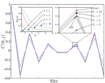
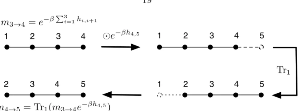
The general idea of the replica method is to approximate the thermal state to a 1-bifactor state in which the QBP can be run directly and is guaranteed to converge in the absence of loops. In the first step, a Trotter-Suzuki (TS) decomposition is used to approximate a thermal state to the state of an Nτ-bifactor with finiteNτ.
Sliding Window
As in the classical setting (2.9), these message-passing rules can be generalized to arbitrary graphs, enabling the calculation of one- and two-body beliefs, from which various quantities of interest, such as energy, can be calculated.
Numerical Results
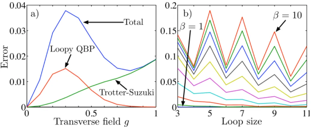
Intuitively, one expects a local algorithm such as belief propagation to be relatively insensitive to the large-scale structure of the graph. We expect QBP to share this property, and Figure 2.5b illustrates the effect of loop size on the mean relative error of the correlation function.
Conclusion
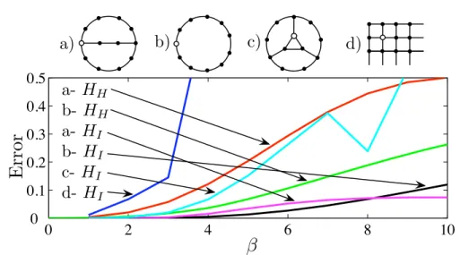
In the classical setting, it has been argued that the physics of random Bethe lattices and Cayley trees is very different [24]. We note that the randomness in quenched disordered systems should not affect the performance of QBP.
Introduction
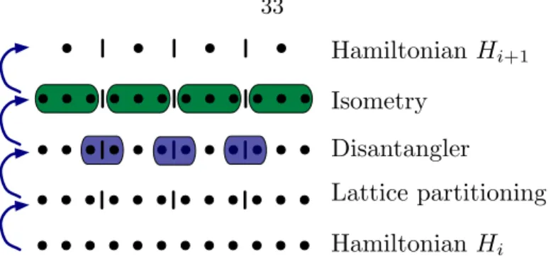
Starting at high temperatures where ordinary BP is accurate, the temperature is lowered until the coarse-grained grid becomes favorable through the elimination of its shortest length-scale degrees of freedom. The coarse-grained procedure is continued as the temperature is lowered to zero where ordinary ER is accurate.
Errors in Belief Propagation Results
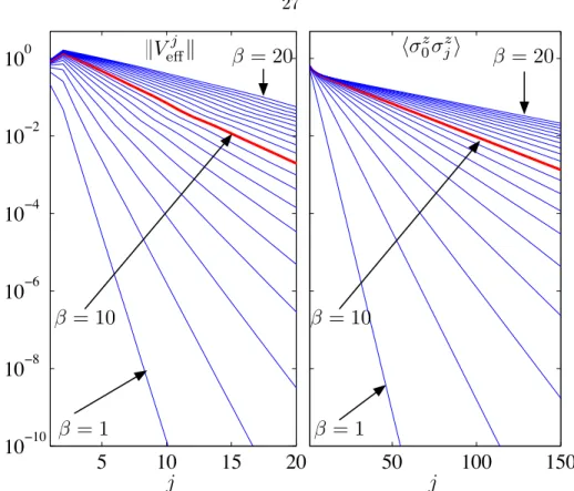
An estimate of the error caused by BP can be used to determine the temperatures at which each coarse-grained procedure should be performed. Upper bound on||Veffj ||(left) and correlations (right) of the Ising chain with critical transverse field.
Disordered System Revisited
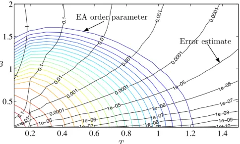
To further reduce finite-size effects, the order parameter EA is evaluated only at the central mesh rotation, away from the boundary. Note, however, that statistical fluctuations of the extinction mean are not included in this error estimate.
Multiscale Entanglement Renormalization
Moreover, this occurs in the region of the phase diagram where the BP error is large. Two examples of MERA structures: For the periodic chain qudit (at the bottom of the figure), a variational family of states is obtained by changing the contents of the fields. Given the MERA structure as shown in Figure 3.6, we have described a recipe that yields a variational family of states for a chain of N d-dimensional qudits parameterized by isometries of the form W: (Cd)⊗n→(Cd)⊗m( constants n≥m depending on the MERA-structure).
Coarse-Grained Belief Propagation
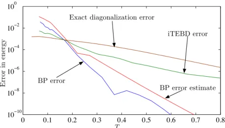
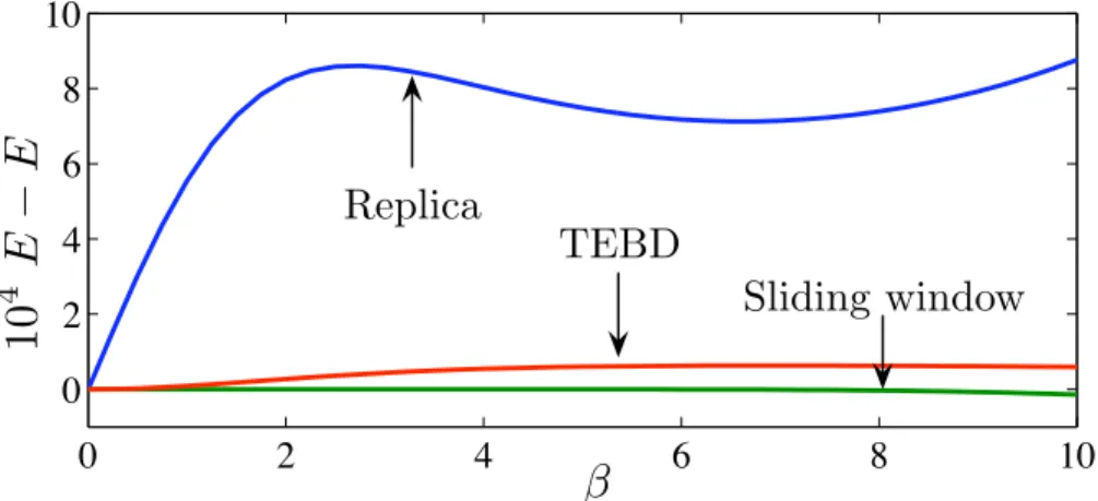
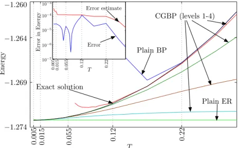
The labels on the temperature axis correspond to the transition temperatures between different levels of coarse particles in the CGBP algorithm. We define δxBPi (T) to be the error attributed to BP at the tenth coarse-grained level. With equal computational costs - which are O(χ3l) - the results are qualitatively equivalent in the sense that they have roughly equivalent maximum error.
Discussion
In the context of the latter, it is natural to study paradigmatic models, such as one-dimensional chains. More generally, it provides procedures for computing the relevant conformal field theory (CFT) parameters in the continuum limit. While such procedures are also available for other variational methods (e.g., matrix product states with transfer matrix methods), they are particularly natural in the present context due to the scale-invariant form of the ansatz .
Anyonic States and Operators
A Unified Treatment of Topological Order
In section 4.2 we give some background on uniionic systems and their description in terms of fusion diagrams. In section 4.4 we apply the ansatz to the golden chain and identify a renormalization group fixed point. It is required to satisfy a number of consistency conditions (see e.g. [51]) the most important of which express associativity of merging and compatibility of merging with braiding.
The Anyonic Hilbert Space and Anyon Diagrams
- Anyons on a disc
- Anyons on a torus
Additional properties such as unity impose further conditions on the shape of the map/matrixU~aa~0(c) for each c. Here we are interested in periodic chains of any arranged on a line, and some modifications of the above formalism are necessary. The representation of the brah~a,~b|n of the vector in (4.12) is again obtained by inverting the diagram and reversing the arrows, i.e.
Anyonic Hamiltonians: Long-range Effective Theories
They can be thought of as describing the dynamics of the internal degrees of freedom of each person fixed on the fixed page.
Anyonic Entanglement Renormalization
- The Setting
- The Ansatz
- Efficient Evaluation of Physical Quantities
- Computational Cost and Refinements of the Ansatz
- Example: Fibonacci Anyons
- Distillable States for Composite Anyon Coding
The same applies to two-point correlation functions for certain distances from the points related to the MERA structure. The rest of this story is the same as that of the MERA for spinning chains, and we refer to the extensive literature (e.g. [39]) on this topic. This determines the shape of the state |ϕni ∈ Hchain,n which corresponds to the upper box in structures as in figure 3.6 (a) and (b), respectively.
Application to the Golden Chain and the Majumdar-Ghosh Chain
The Model
They can be represented by an arbitrary renormalization ansatz (corresponding to the preparation scheme) with the following properties: the state at the top is fixed at |ϕi, and all adjoints of isometrics W† can be implemented by braiding and fusion. There are two extended critical phases for which an exact mapping has been made to the 3-state Potts and tricritical Ising models at the FM and AFM gold chain points respectively [76]. The Majumdar-Ghosh (MG) chain [105] is a model of SU(2) spin 1/2 particles arranged on a chain, where interactions between three particles favor either total spin 3/2 (ferromagnetic/ called FM) or 1/2 (called antiferromagnetic/AFM).
![Figure 4.1. Phase diagram of the model in (4.35) as obtained in [106]. Phases I and II are gapped, with the exact ground states known at the Majumdar-Ghosh (MG) point θ = 3π/2 (see Section 4.4.2) and at tan θ = φ/2](https://thumb-ap.123doks.com/thumbv2/123dok/11220215.0/73.918.335.637.81.349/figure-phase-diagram-obtained-phases-gapped-majumdar-section.webp)
Exact Renormalization Group Fixed Point at the Majumdar-Ghosh
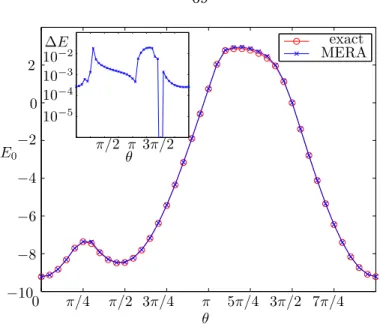
Instead, we limit ourselves to a few example calculations that illustrate the power of the anionic MERA approach. This completes the specification of the MERA to translation (which we correct later), since the top-level state |ϕi depends on the actual state under consideration. This is most easily seen for the state |1τ1τ1τ· · ·i using the diagrammatic calculation: applying a layer (adjoints of) isometries corresponds to stacking N/4 parallel copies of (4.37) above -on the condition.
Numerical Variation over Ansatz States
Two-point correlation function C(r) (cf. 4.39)) of the local topological charge density at the AFM point. Two-point correlation function C(r) (cf. 4.39)) of the local topological charge density at the FM point. Note that at the Majumdar-Ghosh point (θ= 3π/2), the plotted|δC| large, although MERA accurately represents one of the ground states.
Braiding and More General Arrangements of Anyons
The inset illustrates the relative error of the MERA versus the CFT forecast. The two-chain ladder is one of the simplest examples where transpositions must be used to define physically interesting Hamiltonians. The fact that (4.42) is a multi-anyon non-local operator now seems to be an obstacle to the use of the anyonic entanglement renormalization ansatz.
Conclusions
This function is the same as Fermionic Tensor Grids/MERA, where the number of swaps needs to be monitored. The time complexity of our method for one-dimensional systems is dominated by the quantity Nkhk/T, where N is the number of subsystems, T is the temperature, and khki is the limit of the operator norm of the local terms of the Hamiltonian, the interaction strength. A quantum computer's memory simply scales up by N, an exponential improvement over general classical algorithms.
Thermalization Using Phase Estimation
Dimension Reduction Overview
Using this, we can bound the trace norm of the first-order term in the expansion directly. The distribution of the number of operations is known in the theory of success runs. We now assume access to the HamiltonianH and account for the effects of the errors inherent in the phase estimation algorithm.
Perturbative Hamiltonian Update
Perturbative Update with Perfect Operations
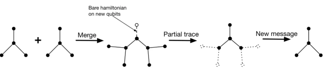
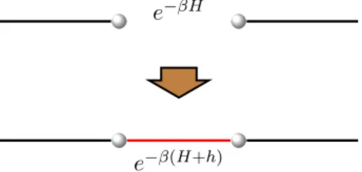
We now give an algorithm that, assuming perfect phase estimation and perfect dephasing, updates the state ρ ∝ e−βH v ρ() ∝ e−β(H+h) to first order in βkhk. The standard procedure for developing from an eigenbasis of an operator to an eigenbasis of a related operator is to use the adiabatic approximation. For this proof it is more convenient to work in the eigenbasis of the new Hamiltonian, H+h.
Concatenation
Errors and Cost of Operations with Finite Precision
For similar energies, the previous map already performs an appropriate update, including updating its own base. If we now forget about the phase estimation result which means partial trace. The vectors |Ei are binary representations of the energy contained in the high-precision phase estimation ancels.
Time Requirements
If you are interested in thermalizing a classical system with a small quantum perturbation, you can first solve the classical part of the Hamiltonian. In the remainder of this dissertation we focused on alternative approximation schemes that improved the efficiency of the previously known methods. The common point of the algorithms discussed in this thesis is the fact that they exploit the location of physical Hamiltonians.
Conclusion