In the first part of this thesis, we investigate the structure of the low-energy subspaces of quantum many-body systems. Preskill, "The ghost in the radiation: Robust encodings of the black hole interior," Journal of High Energy Physics, no.
INTRODUCTION
Low Energies
This again motivates a study of quantum error correction within low-energy subspaces of a quantum system. In Chapter 2, we study the quantum error detection properties associated with low-energy subspaces of a quantum many-body system.
High Energies
A sharpened version of the black hole information problem, the so-called Black Hole Firewall paradox, was presented. We start with a pure state|𝜓i𝑀 that represents the state of the black hole on a first time slice.
BIBLIOGRAPHY
Shaghoulian, ‘Replica wormgaten en de entropie van havikstraling’, Journal of High Energy Physics, nr.
Low Energies
QUANTUM ERROR-DETECTION AT LOW ENERGIES
Introduction
The key to many of these results in the context of topological order and AdS/CFT holographic duality is the language of tensor networks. A similar success story for the use of tensor networks is emerging in AdS/CFT duality.
Our Contribution
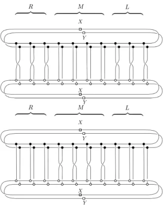
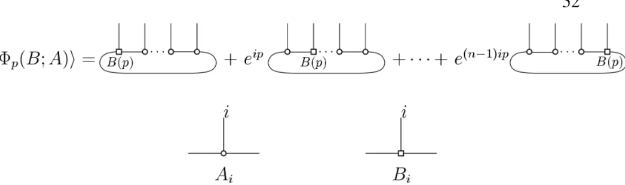
This is due to the exponential decay of the correlation [61]–[63] and the lack of topological order without symmetry protection [18], [64]. Let 𝐴, 𝐵(𝑝) be the tensors associated with the injective excited anzatz state|Φ𝑝(𝐵;𝐴)i, where 𝑝 is the momentum of the state quantity.
Approximate Quantum Error-Detection
- Operational Definition of Approximate Error-Detection
- Necessary Conditions for Approximate Quantum Error-Detection Here we give a partial converse to Corollary 2.3.4, which shows that a condition of
Nevertheless, we show below that, at least for probabilistic noise, simple sufficient conditions for quantum error detection involving only single Kraus operators can be given. Unfortunately, good bounds of the form (2.3.2) are not easy to determine in the cases under consideration.
On Expectation Values of Local Operators in MPS
- Transfer Matrix Techniques
One proceeds as follows: given an injective MPS, let denote the unique fixed point of the transfer operatorE. For the second claim, recall that the power inputs𝑚 of a Jordan block are ( (𝜆 𝐼ℎ+𝑁)𝑚)𝑝,𝑞.
No-Go Theorem: Degenerate Ground Spaces of Gapped Hamiltonians are Constant-Distance AQEDCare Constant-Distance AQEDC
For 𝑘 >2 the inequality follows from the inequality for𝑘 =2 and the submultiplicity of the Frobenius norm due to 2 is the second largest eigenvalue of the transfer operator 𝐸 = 𝐸(𝐴) and where𝑐 is a constant that depends only on the minimal eigenvalue of 𝐸 and the bond dimension𝐷.
AQEDC at Low Energies: The Excitation Ansatz
- MPS Tangent Space Methods: The Excitation Ansatz
- The Norm of an Excitation Ansatz State
- Matrix Elements of Local Operators in the Excitation Ansatz Overview of the ProofOverview of the Proof
- The Parameters of Codes Based on the Excitation Ansatz
For the proof of Lemma 2.6.3 (and other arguments below), we make repeated use of the following statements. Finally, we require a strengthening of the estimates obtained in Lemma 2.6.5, because we are ultimately interested in generating ansatz states: these are superpositions of. 𝐼⊗Δ⊗𝐹𝜏(𝑞)⊗𝐼⊗Δ(𝑗 , 𝑝,ˆ 𝑗ˆ0, 𝑝0) incorporates Δ of the associated transfer operators𝐸 =𝐸𝐸, at least, to the left of the left-hand side of 𝐸.
The cyclicity of the trace allows these to be consolidated into a single term𝐸𝑠 with 𝑠 ≥ 2Δ. The Jordan decomposition𝐸 =|𝑟iihhℓ| inserting ⊕𝐸˜, we obtain. Let 𝐴, 𝐵 be tensors associated with an injective excitation ansatz state |Φ𝑝(𝐵;𝐴)i, where𝑝 is the momentum of the state.
AQEDC at Low Energies: An Integrable Model
- The XXX-Model and the Magnon Code
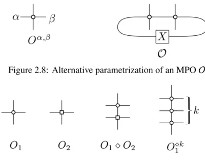
- Matrix Product Operators
- MPS/MPO Representation of the Magnon States
- A Compressed MPS/MPO Representation of the Magnon States
- Action of the Symmetric Group on the Magnon States
- The Transfer Operator of the Magnon States and its Jordan Structure We are ultimately interested in matrix elements hΨ 𝑟 | ( 𝐹 ⊗ 𝐼 ⊗( 𝑛 − 𝑑 ) ) |Ψ 𝑠 i where 𝐹 ∈
- Matrix Elements of Magnon States
- The Parameters of the Magnon code Our main result is the following:Our main result is the following
Specifically, we consider subspaces spanned by states of the form {𝑆𝑟−|Ψi}𝑟 for appropriate choices of magnetization 𝑟. Here we give an MPS/MPO representation of the magnon states that we use throughout our analysis below. It follows that the “descendants”|Ψ𝑠i=𝑆𝑠−|Ψica can be represented as in Figure 2.17, that is, they are MPS of the form.
According to the MPO representation (2.7.4) of 𝑆𝑠−, the matrix elements of this operator can be expressed as Note that in the standard basis spin-𝑗-representation, the lift operator 𝐽+ is strictly lower diagonal.
OBSTACLES TO STATE PREPARATION AND VARIATIONAL OPTIMIZATION FROM SYMMETRY PROTECTION
Introduction
Here, dist(𝑆, 𝑆0) is the Hamming distance, that is, the minimum number of bit flips required to get from 𝑆 to 𝑆0. Fix a family of degree-3 expanders{𝐺𝑛}𝑛∈I and define𝐻𝑛as the ferromagnetic Ising model on the graph𝐺𝑛, i.e. 3.2.2) coincides with the approximation ratio, i.e. the ratio between the expected cost value of Max. (optimal) level-𝑝 variation mode and the maximum slice size.
Corollary 3.2.2 thus provides an explicit upper bound for the approximation ratio achieved by level QAOA. If 𝑝 and 𝐷 are constants, the unitary 𝑈(𝛽, 𝛾) can be realized by a circuit of constant depth composed of nearest neighbors, that is, the circuit is geometrically local.
The Recursive Quantum Approximate Optimization Algorithm
Suppose one prepares the state𝑉|+𝑛and measures a pair of qubits 𝑗 < 𝑘 in the standard basis. The remaining instance of the problem with 𝑛𝑐 variables is then solved by a purely classical algorithm (for example, by a brute force method). Imposing a constraint of the form (3.11) can be seen as rounding correlations between the variables 𝑍𝑖 and 𝑍𝑗. The restriction actually requires these variables to be perfectly correlated or anti-correlated.
We compare the performance of the standard QAOA, RQAOA and local classical algorithms using the Ising Hamiltonians in Eq. 1 defined on the cycle chart. For every integer 𝑛divisible by 6, there exists a family of 2𝑛/3Isend Hamiltonians of the form 𝐻𝑛 = Í. Figure 3.1: Comparisons of level-1 RQAOA and the Goemans-Williamson Algorithm. a) Approximation ratios achieved by level-1 RQAOA (blue) and the Goemans-Williamson (GW) algorithm [21] (red) for 15 instances of the Ising cost function with random ±1 couplings defined on the 2D toric grid of size 16 × 16.
![Figure 3.1: Comparisons of level-1 RQAOA and the Goemans-Williamson Al- Al-gorithm. (a) Approximation ratios achieved by level-1 RQAOA (blue) and the Goemans-Williamson (GW) algorithm [21] (red) for 15 instances of the Ising cost function with random ± 1 c](https://thumb-ap.123doks.com/thumbv2/123dok/10412514.0/132.918.154.771.119.384/comparisons-goemans-williamson-approximation-achieved-williamson-algorithm-instances.webp)
Variable Elimination
Furthermore, any maximum of If a global maximum𝑥 of𝐶(𝑥) happens to satisfy (C.1), the new reduced problem yields a solution to the original problem.
Correlation Rounding
Imposing a constraint of the form (C.1) can be seen as rounding correlations between the variables {𝑥𝑤}𝑤∈𝑓: the constraint indeed requires that for 𝑣 ∈ 𝑓 the variable 𝑥𝑣en𝑥(𝑓\{𝑣}) must be perfect correlated or anti-correlated.
The Recursive QAOA ( RQAOA ) Algorithm
Classical Simulability of Level- 1 RQAOA for Ising Models
The Monte Carlo simulator features runtime scaling in a polynomial manner with the number of qubits, the number of terms in the cost function and the inverse fault tolerance, see [31]. In contrast, RQAOA only requires measurements of a few qubits to estimate the average values of individual terms in the cost function. In this section we discuss another limitation of QAOA that arises from its locality and the covariance condition discussed in Lemma 3.A.2: we compare QAOA with a certain very simple classical local algorithm (see Lemma 3.D.1 below ).
The family (choice){𝑔𝑣}𝑣∈𝑉 can be considered as a set of variational parameters for the classical algorithm. We say that a 𝑟-local classical algorithm is uniform if (by this identification) 𝑔𝑣 ≡ 𝑔 for all 𝑣 ∈𝑉, i.e. if there is a single function𝑔 : R𝐸𝑟(𝑣∗) → {0,1} that determines the behavior of the algorithm .
RQAOA on the Ising Ring
Verstraete, “Lieb-Robinson limits and the generation of correlations and quantum topological ordering,” Physical Review Letters, vol. Hastings, "Quantum systems on non-k-hyperfinite complexes: A generalization of classical statistical mechanics to expanding graphs," Information and Quantum Computation, vol. Hastings, "Trivial low-energy states for motional Hamiltonians, and the quantum pcp conjecture," Information and Quantum Computation, vol.
Raussendorf, "Two-dimensional Affleck-Kennedy- Lieb-Tasaki state on the honeycomb lattice is a universal resource for quantum computation," Physical Review A, vol. Miyake, “Resource quality of a symmetry-protected topologically ordered phase for quantum computation,” Physical Review Letters , vol.
High Energies
BUILDING BULK GEOMETRY FROM THE TENSOR RADON TRANSFORM
Introduction
One such challenge in the AdS/CFT duality is to understand how the boundary degrees of freedom without gravity can reorganize themselves into a higher dimensional bulk configuration with gravity. In general, we do not expect all quantum states from the boundary CFT to correspond to well-defined semi-classical geometries in the bulk. In this paper, we study the above issues in the context of AdS3/CFT2 using an approach based on the tensor Radon transform.
We find that the free fermion ground states in the presence of disorder and a massive deformation do not correspond to a well-defined bulk geometry. In the case where the dynamics is turbulent, we find that the bulk description is qualitatively consistent with a falling spherical shell of massive matter experiencing gravitational pull.
Boundary Rigidity and Bulk Metric Reconstruction
Throughout, we work exclusively in the perturbative regime, to leading order in ℎ, which allows us to relate geodesic length deformations to the Radon transform through (4.2). Before proceeding with the inversion process, we need to understand the inverse Radon transform. Physically, any Radon transform of a pure gauge deformation that reduces to the identity at the limit is zero.
The presence of this kernel is natural because the transform relates geodesic lengths (which are gauge invariant) to metric tensors (which are not), so the Radon transform can only be injective up to gauge. See Appendix 4.B for a more detailed description of the gauge constraints and the radon transform on a hyperbolic background.
Numerical Methods for Reconstruction
- Discretization and Optimization Procedures
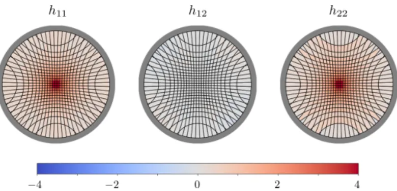
To each tile T in the bulk we associate a tensor ℎ𝑖 𝑗(T ), and for each interval 𝐴 on the boundary we associate a geodesic (of the background metric) 𝛾𝐴 anchored on the endpoints of the interval. Each geodesic anchored at the endpoints of an interval generates a linear equation via the discretized version of the Radon transform (4.2), defined by. We give the full details of the meter setting conditions and the associated partial differential equations in Appendix 4.C.
Reconstruction of the metric perturbation then corresponds to finding the solution to the linear equations (4.3.1) above, subject to the linear constraints (4.3.1). This can be due to a variety of reasons, such as the presence of discretization errors, or if the boundary data are simply inconsistent with a geometric bulk, i.e. if the boundary entropy function does not lie within the range of the forward Radon transform.
Reconstructed Geometries
- Holographic Reconstructions
- Random Disorder
The entanglement propagation wavefront is reflected in the mass as a spherically symmetric disturbance moving from the boundary towards the center. Then we should restore the fact that the corrected geodesics avoid the central region of mass. To fix our background geometry, we numerically calculate the ground state entanglement of the critical Hamiltonian ˆ𝐻.
The large error of reconstruction can be seen as a feature of the fact that the underlying condition is non-geometric. Finally, we can look at the geometries resulting from a random perturbation of the free fermion system.
Geometry Detection
This is most noticeable in the global damping dynamics, where the relative error decreases as the entanglement propagates. However, due to integrability, the state cannot actually be thermalized; the system is subsequently retried and the relative error is returned. At this point, it is not entirely clear why the global damping states have such a small relative error at intermediate times.
In summary, we find that the relative boundary error provides a useful measure of the extent to which a state is geometric or non-geometric. Furthermore, quench dynamics reveal large patterns of geometric evolution, despite the states themselves being non-geometric as characterized by the relative error.
Discussion
We will not comment much on the scope of the tensor Radon transform except to note that the tensor Radon transform is not surjective in general. A useful analytical characterization of the region remains an open problem for the tensor Radon transform on generic manifolds. In this way, we can consider the image of the Radon transformation as a function on the space of boundary subregions.
The transport equation can therefore be seen as the differential form of the Radon transform. We also need to discretize the (ideal) boundary of the Poincaré disk for the Radon transform.