and Future Climate and
II. Sensitivity of Multiangle Imaging to the Optical and Microphysical Properties of Biomass Burning Aerosols
Thesis by
Wei-Ting Chen
In Partial Fulfillment of the Requirements for the Degree of
Doctor of Philosophy
California Institute of Technology Pasadena, California
2009
(Defended December 3, 2008)
© 2009 Wei-Ting Chen All Rights Reserved
Acknowledgements
The past six and half years in Caltech have become an amazing and life-changing journey. It not only enables me to acquire the fundamental knowledge and proper attitudes of conducting scientific research, but also reveals to me the beauty and wonder of our Great Nature. There are many people who made this journey easier and pleasant by kindly offering their invaluable guidance, inspiration, and companionship.
First and the greatest gratitude to my thesis advisor, Prof. John Seinfeld, who is the most supportive supervisor I can ever imagine. His perpetual enthusiasm for science has motivated me, and he is always accessible and delight to help the students with our studies and research, providing his unmatched experience and superb knowledge.
Special thanks go to Dr. Ralph Kahn, my advisor of the MISR project. Dr. Kahn is always patient, thoughtful, and encouraging. He taught me the sound science of aerosol retrievals, and, as an outstanding and dedicated scientist, he also sets a great role model for me.
I would also like to acknowledge my thesis committee: Prof. Paul Wennberg, Prof.
Tapio Schneider, and Prof. Yuk Lin Yung, for their guidance and care during these years.
The projects in this thesis were accomplished with tremendous assistance from many colleagues and peers: Prof. Hong Liao, Prof. Thanos Nenes, Prof. Peter Adams, Dr.
Serena Chung, Dr. Loretta Mickley, Dr. David Nelson, Wen-Hao Li, Kevin Yau, and Dr.
Barbara Gaitley. They have given their rich knowledge, excellent ideas, and precious time to help me solve numerous problems.
I am fortunate to have joined a wonderful research group. I received many help and inspiring inputs from the “modelers” in the Seinfeld group: Havala Pye, Amir Hakami, Daven Henze, Philip Stier, Yi-Chun Jean Chen, and Zachary Lebo, especially during our
“secret coffee meetings”. I am also grateful to the other members in our group for their friendship in these years, especially Sally Ng and Julia Lu. In addition, I appreciate the help from our secretaries Ann Hilgenfeldr, Yvette Grant, Linda Scott, and Dian Buchness, who have made my research work at Caltech hassle-free.
My life in Southern California is enriched by many great friends: Yu Wang, Nina Lin, Hao-Teh Hsu, Hsin-Ling Wang, Jui-Lin Li, Hsi-Yen Ma, Chia-Chun Wu, Chien-Min Wu, Wei-Ju Chen, Chih-Yung Lee, Betsy Wang, my yoga teacher Nancy, and everyone in the Caltech Glee Clubs. My thoughts also go to many old friends in Taiwan: Sue-Ping Liu, Ko-Li Cheng, Meng-Shan Lu, Shu-Han Lin, and my high school teacher Yu-Ya Wu.
Their friendships never fade even though we have been physically parted thousands of miles away. I would also like to thank Prof. Jen-Ping Chen at National Taiwan University for advising my undergraduate study and encouraging me to study abroad.
Lastly, but most importantly, I am grateful to the unconditional love and unwavering trust from my dear parents, Liang-Kuang Chen and Chin-Hsiu Szu, grandmother, Yuk- Tong Ou, brother, Wei-Teh Chen, and my life-companion, Eh Tan. To them I sincerely dedicate this thesis. My family members in Taiwan, Hong Kong, Indonesia, Canada, and the United States also show tireless support to my pursuit of the degree. I want to express the deepest gratitude to them from the bottom of my heart.
Abstract
To understand the interaction between aerosols and climate, equilibrium simulations with a general circulation model are carried out in Part I to study the effects of future climate change on aerosol distributions, as well as the climate responses to future aerosol changes. The predicted warmer climate induced by carbon dioxide modifies the climate- sensitive emissions, alters the thermodynamic partitioning, and enhances wet removal of the aerosols. The direct radiative perturbations of aerosols, and the modification of clouds by aerosols can potentially change the temperature distribution, the hydrological cycle, and the atmospheric circulation; the pattern of climatic impacts from aerosols are differentiated from those of anthropogenic greenhouse gases. In Part II, the aerosol retrieval algorithm of the remote sensing instrument, the Multi-angle Imaging SpectroRadiometer (MISR), is assessed for the retrieval of biomass burning aerosols. By comparisons with coincident ground measurements and theoretical sensitivity tests, specific refinements to particle and mixture properties assumed in the algorithm for biomass burning aerosols are proposed. Representative case studies confirm the theoretical results and underline the key role of surface characterization in the remote sensing of aerosols.
Table of Contents
Acknowledgements ...iii
Abstract... v
Table of Contents ... vi
List of Figures ...ix
List of Tables ... xv
Chapter 1 Introduction ... 1
Part I. Global Simulations of Interactions between Aerosols and Future Climate ... 7
Chapter 2 Roles of Climate Change in Global Predictions of Future Tropospheric Ozone and Aerosols ... 8
Abstract... 9
2.1 Introduction ... 11
2.2 Model Description and Experimental Design ... 14
2.2.1 The Unified Model ... 14
2.2.2 Climate Simulations... 16
2.2.3 Chemistry Simulations... 17
2.2.4 Emission Inventories... 19
2.3 Predicted Climate Change... 20
2.3.1 Predicted Changes in Temperature... 21
2.3.2 Predicted Changes in Hydrological Cycle ... 21
2.3.3 Predicted Changes in Winds ... 22
2.4 Effects of CO2-Driven Climate Change on Tropospheric Ozone and Aerosols ... 24
2.4.1 Predicted Changes in Ozone ... 24
2.4.2 Predicted Changes in Carbonaceous Aerosols ... 26
2.4.3 Predicted Changes in Sulfate and Nitrate Aerosols... 27
2.4.4 Predicted Changes in Sea Salt and Mineral Dust ... 29
2.4.5 Effects of Climate Change in the Presence of Heterogeneous Reactions... 31
2.5 Predicted O3 and Aerosol Concentrations with Year 2100 Projected Emissions and Climate... 33
2.6 Impact of Climate Change on Estimates of Year 2100 Direct Radiative Forcing ... 35
2.7 Summary and Discussion... 38
References... 42
Chapter 3 Future Climate Impacts of Direct Radiative Forcing of Anthropogenic Aerosols, Tropospheric Ozone, and Long-lived Greenhouse Gases ... 68
Abstract... 69
3.1 Introduction ... 71
3.2 Model Description and Experimental Design ... 73
3.2.1 The Unified Model ... 73
3.2.2 Climate Simulations... 74
3.2.3 Present-day and Year 2100 Anthropogenic Aerosols, Tropospheric Ozone, and Greenhouse Gases ... 76
3.3 Estimated Changes in Global Climate ... 80
3.3.1 Surface Air Temperature... 80
3.3.2 Tropospheric Temperature and Stability... 82
3.3.3 Global Circulation ... 83
3.3.4 Hydrological Cycle ... 85
3.3.5 Energy Budgets ... 88
3.4 Estimated Regional Climate Changes in Asia in Winter Ozone and Aerosols ... 89
3.5 Summary and Conclusions... 92
References... 95
Chapter 4 Global Climate Response to Anthropogenic Aerosol Indirect Effects: Present Day and Year 2100 ... 119
Abstract... 120
4.1 Introduction ... 121
4.2 Descriptions of Global Models... 124
4.2.1 CACTUS Unified Model and Offline Aerosol Mass Concentration... 125
4.2.2 GISS-TOMAS Model, FN Activation Parameterization, and Derivation of Aerosol-Nc Relationships ... 128
4.2.3 GISS III GCM and the Modification of Stratiform Cloud Scheme... 131
4.2.3.1 Droplet Effective Radius and Cloud Optical Depth ... 132
4.2.3.2 Autoconversion Rate... 133
4.2.3.3 Aerosol Direct Effect ... 134
4.3 Equilibrium Climate Simulations with GISS III GCM ... 135
4.4 Responses of the Equilibrium Climate to Perturbations of Nc... 139
4.4.1 Predicted Present-Day Equilibrium Climate ... 139
4.4.2 Effects of Change of Nc from Pre-Industrial to Present Day on Equilibrium Climate ... 142
4.4.3 Perturbations of Nc from Present Day to Year 2100 to Equilibrium Climate ... 146
4.5 Predicted Equilibrium Climate Response From Present Day to Year 2100 to the Combined Effects of GHG, ADE and AIE ... 148
4.6 Climate Sensitivities and Hydrological Sensitivities for ADE, AIE, and GHG: Comparing the Present work with Previous Related Studies... 150
4.7 Summary and Conclusions... 152
References... 156
Part II. Sensitivity of Multiangle Imaging to the Optical and Microphysical Properties of Biomass Burning Aerosols... 184
Chapter 5 Sensitivity of Multiangle Imaging to the Optical and Microphysical Properties of Biomass Burning Aerosols ... 185
Abstract... 186
5.1 Introduction ... 187
5.2 Near-Coincident MISR-AERONET Measurements in Major BB Regions... 190
5.2.1 Data Selection... 190
5.2.2 Comparison of Near-coincident MISR-AERONET BB Cases ... 192
5.3 BB Particle Property Characterization... 199
5.4 Theoretical Sensitivity Study for BB Aerosol Components ... 203
5.4.1 BB Aerosol Components and Mixing Groups ... 204
5.4.2 Radiative Transfer Simulations, and the 2 Test Variables for Evaluating Agreement Between Simulated Reflectances in the Sensitivity Test... 205
5.4.3 Results of MISR Theoretical Sensitivity to BB Components ... 207
5.5 MISR Research Retrieval Study of Field Cases with Proposed BB Components and Detailed Surface Characterization ... 211
5.5.1 Patches and Surface Characterization for Selected Field Cases... 212
5.5.2 MISR Research Retrievals of Selected Field Cases ... 214
5.6 Summary and Conclusions... 223
References... 228
List of Figures
Figure 2-1. Temperature responses in the equilibrium climate to the increase in CO2
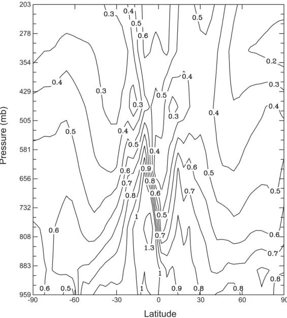
concentration from 368 ppmv in year 2000 to 836 ppmv in year 2100, including predicted changes (°C) in (a) annual mean surface air temperature and (b) zonal annual mean atmospheric temperature. The global mean value is indicated at the top right corner of Figure 2-1a... 56 Figure 2-2. (a) Predicted year 2000 zonal annual mean equilibrium specific humidity
(g-H2O kg-air–1) as a function of pressure. (b) Predicted changes in zonal annual mean equilibrium specific humidity (g-H2O kg-air–1) relative to year 2000. (c) Predicted changes (mm day–1) relative to year 2000 in annual mean precipitation. (d) Predicted changes (mm day–1) relative to year 2000 in zonal annual mean precipitation. The global mean value is indicated at the top right corner of Figure 2-2c. ... 57 Figure 2-3. Latitude-pressure distributions of zonal and seasonal mean (a) present-day
vertical velocity (10–5 mb s–1), (b) changes in vertical velocity (10–5 mb s–1) from year 2000 to year 2100, and (3) changes in mass stream function (1010 kg s–1) from 2000 to 2100. Positive values of the mass stream function
indicate anticlockwise circulation... 58 Figure 2-4. Predicted changes (m s–1) in (a) annual mean surface wind speed and (b)
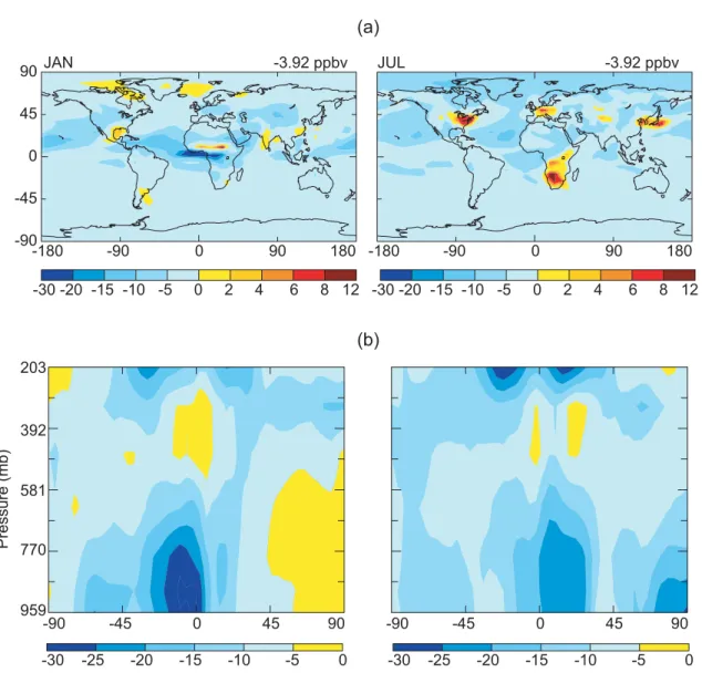
zonal annual mean surface wind speed from 2000 to 2100. The global mean change is indicated for Figure 2-4a. ... 59 Figure 2-5. (a) Changes in January and July predicted surface-layer ozone
concentrations (ppbv, CL2100EM2000 – CL2000EM2000) resulting from CO2-driven equilibrium climate change over 2000–2100. Global mean change is indicated at the top right corner of each panel. (b) Percentage changes ((CL2100EM2000 – CL2000EM2000) 100/CL2000EM2000) in
January and July zonal mean ozone concentrations. ... 60 Figure 2-6. Changes in annual mean concentrations (ng m–3, CL2100EM2000 –
CL2000EM2000) of (a) BC, (b) POA, and (c) SOA at selected layers resulted from the CO2-driven climate change over 2000–2100. Global mean change is indicated at the top right corner of each panel. ... 61 Figure 2-7. (a) Zonal mean changes in OH concentrations (105 radicals cm–3)
resulting from CO2-driven climate change (CL2100EM2000 –
CL2000EM2000). (b) Zonal mean changes in OH concentrations (105 radicals cm–3) resulting from the changes in both climate and emissions
(CL2100EM2100 – CL2000EM2000). Left panels are for January and right panels are for July. ... 62 Figure 2-8. Predicted changes in annual mean sulfate concentration (pptv,
CL2100EM2000 – CL2000EM2000) at the surface layer resulting from CO2- driven climate change from 2000 to 2100. Global mean change is indicated at the top right corner of the panel. ... 63
Figure 2-9. Ratios of the predicted annual and zonal mean nitrate concentrations from CL2100EM2000 to CL2000EM2000. ... 64 Figure 2-10. Annual mean differences between the effects of CO2-driven climate
change in the presence and absence of heterogeneous reactions [(CL2100EM2000h – CL2000EM2000h) – (CL2100EM2000 –
CL2000EM2000)] for the surface-layer concentrations of (a) O3, (b) sulfate, and (c) nitrate. The global mean value is indicated at the top right corner of
each panel... 65 Figure 2-11. (a) Predicted year 2100 surface-layer O3 mixing ratios (ppbv) with
changes in both climate and emissions. (b) Predicted changes in surface-layer O3 mixing ratio (ppbv) from 2000 to 2100. (c) Differences (ppbv) between surface-layer O3 mixing ratios simulated with changes in both climate and emissions and those with changes in emissions only. Top panels are simulated in the absence of the heterogeneous reactions as discussed in the text, while the bottom panels include heterogeneous reactions. The global mean value is indicated at the top right corner of each panel. ... 66 Figure 2-12. (a) Predicted year 2100 surface-layer dry aerosol mass concentrations
(μg m–3) with changes in both climate and emissions. Dry aerosol mass is the sum of sulfate, nitrate, ammonium, BC, POA, and SOA. (b) Predicted changes in surface-layer dry aerosol mass concentrations (μg m–3) from 2000 to 2100.
(c) Differences (μg m–3) between surface-layer dry aerosol mass
concentrations simulated with changes in both climate and emissions and those with changes in emissions only. Top panels are simulated in the absence of the heterogeneous reactions as discussed in the text, while the bottom panels include heterogeneous reactions. The global mean value is indicated at the top right corner of each panel. ... 67 Figure 3-1. Annual and seasonal differences in column concentrations between
present-day and year 2100 for anthropogenic aerosols (mg m–2) and
tropospheric ozone (Dobson Units). (a) Ammonium sulfate (b) Ammonium nitrate (c) POA (d) SOA, (e) BC, and (f) O3 (ANN = annual mean, DJF = seasonal mean over December-January-February, and JJA = seasonal mean
over June-July-August)... 105 Figure 3-2. Annual mean change in instantaneous forcing (W m–2) (a) at tropopause
and (b) at surface imposed by changes of anthropogenic aerosol (left column), tropospheric ozone (middle column), and greenhouse gases (right column)
between present-day and year 2100... 106 Figure 3-3. Latitude-pressure distribution of changes in atmospheric forcing (W m–2)
in (a) DJF and (b) JJA imposed by changes of anthropogenic aerosol,
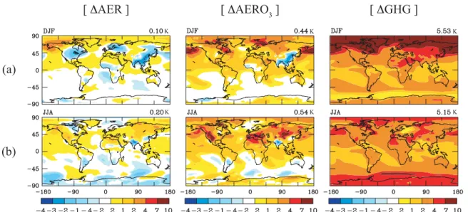
tropospheric ozone, and GHG between present-day and year 2100... 107 Figure 3-4. Predicted change in global surface air temperature (K) in (a) DJF and (b)
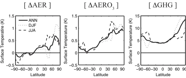
JJA. Note the color scale for GHG differs from the other two. ... 108 Figure 3-5. Predicted zonal mean changes in surface air temperature (K). Note the
vertical scale for GHG differs from the other two. ... 109
Figure 3-6. Latitude-pressure distribution of changes in annual mean temperature (K). 110 Figure 3-7. Latitude-pressure distribution of stream function (1010 kg s–1, positive
values indicate counterclockwise flow) in (a) DJF and (b) JJA, and zonal wind (m s–1, positive values indicate westerlies) in (c) DJF and (d) JJA. Left:
seasonal mean in simulation PD; middle: AER; right: GHG... 111 Figure 3-8. Latitude-pressure distribution of changes in annual mean specific
humidity. (a) Absolute change (g-H2O kg-air–1) and (b) relative change (%).
Note the color scale in (b) differs between AER and GHG. ... 112 Figure 3-9. Predicted zonal mean changes in (a) excess precipitation (total
precipitation minus evaporation, mm day–1) and (b) moist-convective (MC) precipitation (mm day–1). Note the vertical scales differ between AER and GHG. ... 113 Figure 3-10. Predicted zonal mean changes in (a) moist-convective (MC) cloud cover
(%), and (b) high cloud cover (%). Note the vertical scales differ between
AER and GHG... 114 Figure 3-11. Predicted zonal mean changes in (a) net shortwave (SW) flux and (b) net
longwave (LW) flux (W m–2) at TOA. Positive values correspond to
downward fluxes. Note the vertical scales differ between AER and GHG. .. 115 Figure 3-12. Predicted zonal mean changes in surface fluxes (W m–2) of (a) absorbed
(abs.) shortwave radiation (SW, negative values indicate surface solar dimming), (b) sensible heat (SH, positive values indicate flux from atmosphere into surface), and (c) latent heat (LH, positive values indicate decreased evaporation). Note the vertical scales differ between AER and
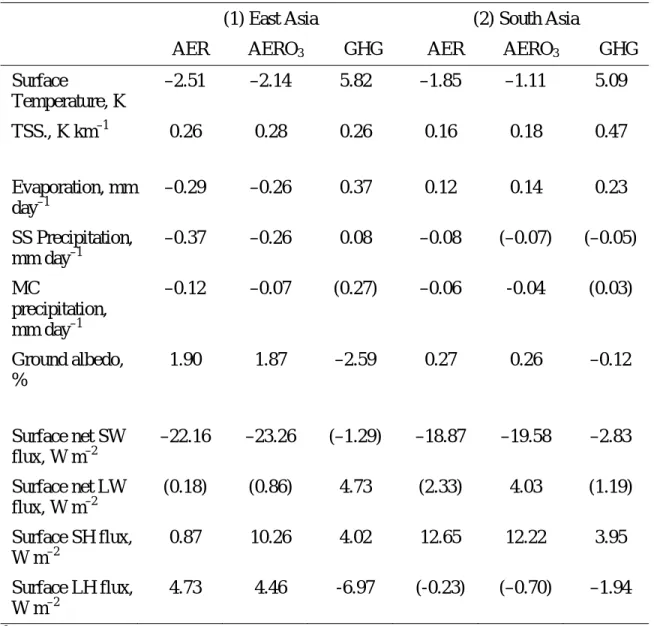
GHG. ... 116 Figure 3-13. Regions (shaded) for calculating the statistics of regional climate change
presented in Table 3-4. (1) East Asia. (2) South Asia. ... 117 Figure 3-14. Predicted change over East and South Asia in DJF (a) in precipitation
(mm day–1) and (b) in sea level pressure (color shading, hPa) and surface wind field (vector, m s–1). Note the color scale differs between AER and GHG. .. 118 Figure 4-1. Schematic diagram for experimental design... 172 Figure 4-2. Annual mean total column burden (mg m–2) of sulfate, nitrate,
ammonium, POA, SOA, and BC for (a) PI, (b) 20C, (c) 21C. Global average values are given in the upper right corner of each panel. ... 173 Figure 4-3. Annual mean column burden of sea salt (mg m–2) for 20C. Global average
values is given in the upper right corner. ... 174 Figure 4-4. The left column shows the changes in annual mean Nc at the lowest
model layer (972 hPa) (a) from PI to 20C and (b) from 20C to 21C. The right column shows the annual mean instantaneous TOA AIE forcing (i.e. changes in TOA cloud forcing) (c) from PI to 20C and (d) from 20C to 21C. Global
average values are given in the upper right corner of each panel ... 175
Figure 4-5. Comparisons of zonal mean cloud properties between predicted present- day equilibrium climate accounting for GHG and anthropogenic aerosol direct and indirect effects (DG20CI20C, solid lines) and satellite observations (dashed lines): (a) column Nc, (retrievals based on ISCCP [Han et al., 1998]) (b) re at cloud top (retrievals based on ISCCP [Han et al., 1994], for year 1987), (c) total cloud fraction (measurements from ISCCP, from July 1986 to June 2006) and (d) SW and LW cloud forcing (measurements from ERBE [Kiehl and Trenberth, 1997]; black lines for shortwave component, and gray lines for longwave component). ... 176 Figure 4-6. Present-day climate response to perturbation of AIE from pre-industrial to
present day (DG20CI20C – DG20CIPI): vertical zonal profiles of changes in annual mean (a) Nc in liquid stratiform clouds (cm–3), (b) total cloud water content (10–6 kg-H2O kg-air–1), (c) re in liquid stratiform clouds (μm) (d) temperature (K), (e) specific humidity (10–4 kg-H2O kg-air–1), and (f) mass stream function (1010 kg s–1, positive values indicate counterclockwise flows);
annual mean changes in (g) Ts (K) and (h) Precipitation (mm day–1). Changes that insignificant relative to the 95% confidence ... 177 Figure 4-7. Present-day climate response to perturbation of AIE from pre-industrial to
present day (DG20CI20C – DG20CIPI): zonal mean changes in (a) Nc at 850 hPa (cm–3), (b) TOA SW CF (W m–2), (c) Ts (K), and (d) Precipitation (mm day–1) (Black solid lines for annual average, gray lines for average over DJF, and
dotted lines for average over JJA). ... 178 Figure 4-8. Similar to Figure 4.6 but for present-day climate response to
perturbation8of AIE from present day to year 2100 (DG20CI21C – DG20CI20C).... 179 Figure 4-9. Similar to Figure 4.7 but for present-day climate response to perturbation
of AIE from present day to year 2100 (DG20CI21C – DG20CI20C). Note the
vertical scales in are different... 180 Figure 4-10. Climate responses to combined effects of GHG and anthropogenic
aerosol direct and indirect effect from present day to year 2100 (DG21CI21C – DG20CI20C): vertical zonal profiles of changes in annual mean (a) total cloud water content (10–6 kg-H2O kg-air–1), (b) temperature (K), and (c) specific humidity (10–4 kg-H2O kg-air–1); annual mean changes in (d) Ts (K) and (e) Precipitation (mm day–1). Global average values are given in the upper right corner of (d) and (e). Note the color scales are different from previous figures. 181 Figure 4-11. Climate responses to combined effects of GHG and anthropogenic
aerosol direct and indirect effect from present day to year 2100 (DG21CI21C – DG20CI20C): zonal mean changes in (a) Ts (K), (b) excess precipitation (total precipitation minus evaporation, mm day–1), and (c) precipitation from stratiform clouds (mm day–1), and vertical zonal profiles of changes in annual mean (d) mass stream function (1010 kg s–1). (In (a)–(c), black solid lines for annual average, gray lines for average over DJF, and dotted lines for average over JJA) ... 182
Figure 4-12. Similar to Figure 4-11, but for climate responses from present day to
year 2100 predicted by the standard version of GISS III (DG21C – DG20C)... 183 Figure 5-1. Comparisons among coincident MISR-AERONET BB cases with mid-
visible AOD>0.15: (a) AERONET mid-visible AOD (AODA) vs. SSA (SSAA), (b) AODA vs. difference in AOD (AODM–A), (c) SSAA vs. difference in SSA (SSAM–A), (d) AODM–A vs. SSAM–A, (e) AERONET Ångstrom Exponent (ÅA) vs. AODM–A, (f) AERONET SSA spectral dependence (0 A) vs. SSAA, (g) ÅA vs. difference in Ångstrom Exponent (ÅM–A), (h) 0 A vs. difference in SSA spectral dependence (0 M–A). In each panel, cases are categorized into four groups (see text for details): black diamonds for group 1, red triangles for group 2, green squares for group 3, and yellow circles for group 4. ... 251 Figure 5-2. The means (vertical lines) and ranges (grey bars) of reported physical and
optical parameter values for haze, aged, and fresh plumes in different regions:
(a) number-weighted geometric mean radius (rpg,N), (b) geometric standard deviation (g), (c) single scattering albedo at 550 nm (0,550), (d) real part of refractive index (nr) at 550 nm, and (e) imaginary part of refractive index (ni) at 550 nm. The vertical lines are red for fresh plumes (< 1 day old), blue for aged plumes (1–3 days old), and green for regional haze (> 3 days old or mixed). (Abbreviations: Afc = Africa, S Am = South America, N Am = North America, C Am = Central America) ... 252 Figure 5-3. Sensitivity results of eight target atmospheric BB components assuming
AOD = 0.2. Each individual sub-plot shows the results for comparisons against one target atmospheric component (marked at the upper-left corner of each sub-plot), with the comparison space rpg,N and 0,558 values organized along the x and y axes, respectively. Overall, the plot array is arranged by the rpg,N and 0,558 of the target atmospheric components (marked at the bottom and the left of the plate). The lower-left sub-plot shows positions of all components on the rpg,N-0,558 plane (green spots). Retrieved component fractions are proportional to the area of colored circles; the gray circle in the lower-left plot is the scale of 100% fraction. For the target atmospheric
component in each panel, the red circle shows the minimum retrieved fraction, and the blue shows the maximum fraction. For the other components, the circle shows only the maximum fraction, and is shaded black if more than 20%, otherwise, gray. Conditions of 1 atm surface pressure and 2.5 m s–1 wind speed, for mid-latitude geometry, over a dark water surface, are assumed in these radiative transfer calculations... 253 Figure 5-4. Same as Figure 5-3, but for atmospheric BB components with having
AOD = 0.5. ... 254 Figure 5-5. Spectral AOD for coincident AERONET measurements (black solid
lines), best-fit MISR v17 Standard Retrievals (black dashed lines), and best-fit Research Retrievals for all patches (gray solid lines for patch with lowest 2, gray dotted lines for patch P0) for the four coincident BB cases. ... 255 Figure 5-6. Normalized number size distributions for coincident AERONET
measurements (green lines), best-fit MISR v17 Standard Retrievals (blue
lines), and best-fit Research Retrievals (red lines for the best patch, yellow lines for P0, and gray lines for patches with 2 < 1.5) for the four coincident BB cases. The best patch is also denoted by ** in the legend. ... 256 Figure 5-7. The third surface RPV parameter retrieved by the MISR v17 Standard
Algorithm at all four MISR channels for hazy day (gray dashed lines) and the clean day orbit (black solid lines) for (a) Ilorin_2001/02/24, (b)
Ouagadougou_2000/12/18, and (c) Ilorin_2001/ 02/17. For each case, plots
are shown for the best patch (left) and for P0 (right)... 257
List of Tables
Table 2-1. Summary of Chemistry Simulations ... 48
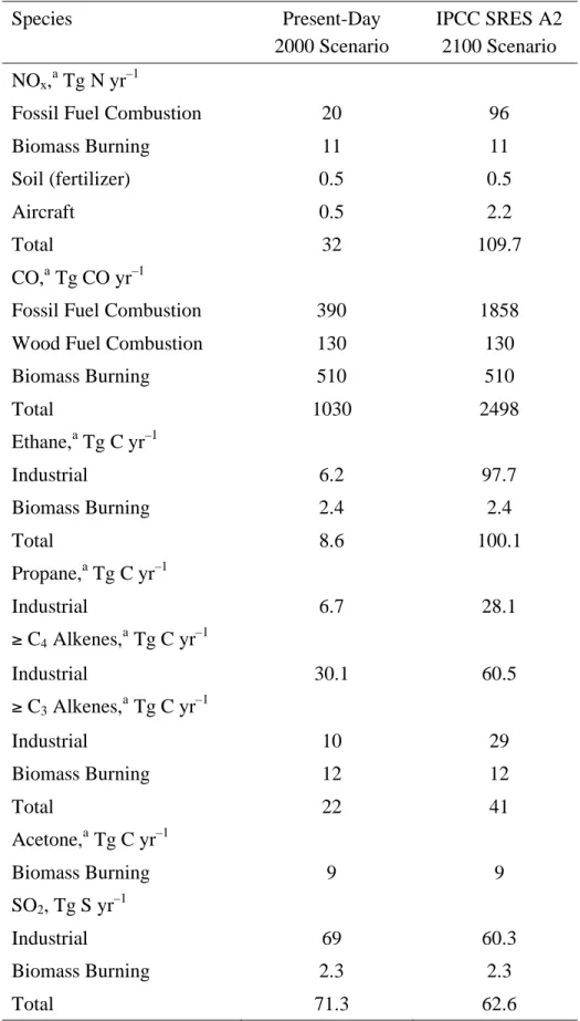
Table 2-2. Global Annual Anthropogenic Emissions for the Years 2000 and 2100 ... 49
Table 2-3. Climate-sensitive Natural Emissions... 51
Table 2-4. Predicted Annual and Global Burdens ... 52
Table 2-5. Global Budget for Tropospheric O3... 53
Table 2-6. Global Budget for Sulfate Aerosol ... 54
Table 2-7. Effect of Climate Change on Estimates of Year 2100 TOA Radiative Forcing... 55
Table 3-1. Summary of Climate Experiments ... 99
Table 3-2. Present-Day (year 2000) and Year 2100 Annual Mean Global Burdens of Anthropogenic Aerosols, Tropospheric Ozone, and Greenhouse Gas Mixing Ratios Used in This Study ... 100
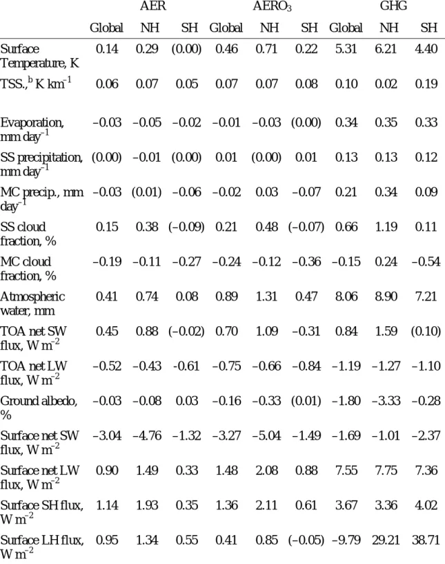
Table 3-3. Global and Hemispherical Annual Mean Differences of Selected Climate Parameters... 101
Table 3-4. Regional Mean Differences of Selected Climate Parameters in DJF over East and South Asia... 103
Table 3 -5. Summary and Comparison of Patterns of Equilibrium Climate Response to Changes of Aerosol Direct Forcing and GHG Forcing from Present Day to Year 2100 Predicted in This Study ... 104
Table 4-1. Global Models in This Study ... 161
Table 4-2. Global Annual Burdens (Tg dry mass) of Aerosols Derived by the Caltech Unified Model ... 162
Table 4-3. Experimental Design of the Equilibrium Simulations with GISS III GCM .. 163
Table 4-4. Global Annual Mean Values of Key Climate Variables in the Present- Day Equilibrium Simulations With and Without Explicit Droplet- Dependence in Stratiform Clouds ... 164
Table 4-5. Comparison of Global Annual Mean Cloud Properties in Present-Day Simulation GD20CI20C With Remote Sensing Observations and Predictions in Selected GCM Studies... 165
Table 4-6. Changes in Annual Mean Cloud Properties Between the Equilibrium Climates ... 166
Table 4-7. Similar to Table 4.6, but for Changes in Annual Mean Temperature, Precipitation, Hydrological Sensitivity, and Surface Radiative Fluxes ... 168
Table 4-8. Change in Global Annual Mean Values of Key Climate Variables Between the Present-day and Year 2100 Equilibrium Simulations, Predicted by the Modified and Standard Version of GISS III ... 169
Table 4-9. Comparisons of Present Day to Year 2100 Forcing and Climate
Response Between the Present Study and Previous Related Studies... 170
Table 4-10. Summary of Patterns of Equilibrium Climate Responses in the Present Study... 171
Table 5-1. AERONET Sites in Major BB Regions Selected for Coincident MISR- AERONET Measurement Comparisons... 235
Table 5-2. Characteristics of Four Groups of BB Cases, Based on Comparisons of AOD and SSA for Coincident MISR-AERONET Measurements ... 236
Table 5-3. BB Aerosol Physical and Optical Property References Covered in This Review of the Field Experiment Literature ... 238
Table 5-4. Profiles of Fresh Plumes, Aged Plumes, and Haze Based on the Literature ... 240
Table 5-5. BB Aerosol Component Models ... 241
Table 5-6. BB Aerosol Mixing Groups ... 242
Table 5-7. Summary of Sensitivity Results for Unimodal BB Particle Cases... 243
Table 5-8. Additional Components Used in the MISR Research Aerosol Retrieval Algorithm for the Four Representative Coincident BB Cases... 245
Table 5-9. Additional Components Used in the MISR Research Aerosol Retrieval Algorithm for the Four Representative Coincident BB Cases... 246
Table 5-10. AOD at 558 nm and Angstrom Exponent from AERONET Measurements, MISR v17 Standard Retrieval and Research Retrieval Results, for the Four Coincident BB Cases ... 247
Table 5-11. Aerosol Fine Mode Fraction, Fine Mode Size, and Coarse Mode Size From AERONET Measurements, MISR v17 Standard Retrievals, and Research Retrieval Results, for the Four Coincident BB Cases ... 248
Table 5-12. Total and Fine Mode SSA and SSA Spectral Dependence From AERONET Measurements, MISR v17 Standard Retrieval, and Research Retrieval Results, for the Four Coincident BB Cases ... 250
Chapter 1
Introduction
Aerosols, suspended fine solid and liquid particles in the atmosphere, are one of the most critical factors controlling Earth’s climate system. Advances in understanding the role of aerosols in the climate system are imperative in the assessment and prediction of climate change. In Part I of this thesis, numerical simulations from a general circulation model are used to systematically explore the important interactions between aerosols and the climate. In Part II, the aerosol retrieval algorithm of a remote sensing instrument is investigated and refined, specifically for the measurements of biomass burning aerosols.
Aerosols can be categorized on the basis of their origins. “Primary aerosols” are those released into the atmosphere directly in the form of particles from natural and anthropogenic sources. Examples of primary aerosols include wind-blown dust particles from soils and deserts, sea salt particles from bursting bubbles in the sea spray, and black carbon and primary organic particles from combustion processes of fossil fuel burning and biomass burning. “Secondary aerosols”, on the other hand, are generated in the atmosphere through physical or chemical transformations of the “precursor” gases.
Important secondary aerosols include sulfate (SO42–
) particles from oxidation of SO2 and the subsequent condensation of sulfuric acid, nitrate (NO3–)particles from the oxidation of NO2 and the subsequent condensation of nitric acid, and secondary organic particles from the oxidation and condensation of biogenic volatile organic compounds (VOC). The formation of secondary aerosols can be very complicated, involving mechanisms such as gas-to-particle conversion (e.g., homogeneous and heterogeneous nucleation), gas phase and liquid phase chemical reactions (e.g., ring-opening processes of aromatic hydrocarbons), and cloud processing.
Changes in climate can affect the emission strength, removal processes, thermodynamic equilibrium, chemical reactions, and the temporal and spatial distributions of aerosols. In turn, aerosols can impact the climate by perturbing the energy balance of the Earth system. The climate and the aerosols thus form a complex feedback system. Numerical experiments with a General Circulation Model (GCM) are one of the key approaches in studying the responses of the climate system to an introduced perturbation (forcing). Transient simulations, in which the perturbation (or forcing) changes along the course of the integration, are usually designed to reproduce current climate conditions or forecasting future climate change. Equilibrium simulations, in which the forcing is held fixed at a certain level during the entire integration, generally result in more pronounced responses than the transient simulation, and are usually chosen to delineate and compare relative impacts of various forcing mechanisms.
In Part I, we use equilibrium simulations with the Goddard Institute for Space Studies (GISS) GCM as our tool to answer the following questions: (1) How will aerosol burden and composition be influenced by future climate change? (2) How will future climate respond to the direct radiative perturbations of aerosols? (3) How will future climate respond to the modifications of clouds by aerosols?
CO2 and the other major greenhouse gases (GHG) are the dominant contributors to current and future climate change. Using a unified climate-chemistry-aerosol model within GISS GCM II’, the effect of future (year 2100) CO2-driven equilibrium climate change on the global distributions of tropospheric ozone, anthropogenic aerosols (sulfate, nitrate, ammonium, black carbon, primary organic carbon, secondary organic carbon), sea salt and dust aerosols is predicted in Chapter 2. Increased CO2 is predicted to lead to
warmer temperature and enhanced precipitation, which increases wet removal, changes emissions that are sensitive to climate, and shifts the thermodynamic partitioning of the aerosols. The changes in future direct radiative forcing associated with the impact of climate change on aerosol burdens are also calculated and compared to those associated with future emission changes.
Aerosols can modify the dominant, long-term, and more spatially homogeneous GHG-induced climate change and create more complexity, especially on a regional basis.
Aerosols directly alter the Earth’s radiative budget by scattering and absorbing sunlight.
This so-called “aerosol direct radiative effect” and its climatic impact is explored in Chapter 3 with the 9-layer GISS GCM II’. Increased aerosol burdens in the atmosphere, through their direct effect, decrease the solar radiation received by the surface, while at the top of the atmospheric column, the net (incident plus reflected) solar flux can be either enhanced or reduced, depending on the relative magnitude of particle scattering versus particle absorption. The radiative perturbation of aerosol direct effect can change the temperature distribution, the strength of the hydrological cycle, and the atmospheric circulations. The characteristics of future equilibrium climate responses to the change in anthropogenic aerosol direct effect, tropospheric ozone, and GHG are analyzed and differentiated.
Aerosols can also indirectly influence the radiation by modifying the amount, reflectivity (albedo), and lifetime of the clouds; these “indirect effects” are studied in Chapter 4. Soluble aerosols may act as cloud condensation nuclei (CCN), controlling the number concentration of cloud droplets. Given the same amount of cloud liquid water, increased droplet number concentrations owing to more abundant aerosols may produce
smaller droplets, thereby leading to higher cloud albedo (i.e., “first indirect effect” or
“cloud albedo effect”). Changes in droplet number concentrations and droplet size distributions also have impacts on the formation of precipitation in the clouds, termed the
“second indirect effect” or “cloud lifetime effect”. In Chapter 4, a new formulation is developed to provide correlations between aerosols and cloud droplet number concentrations, and the 23-layer GISS GCM III is modified to include processes related to aerosol indirect effects in the stratiform clouds. The equilibrium climate responses to indirect effects between pre-industrial and present day, and between present day to year 2100, are diagnosed and compared to the climate responses to GHG and aerosol direct effect.
The climatic impacts of aerosols are determined by the abundance, size, chemical composition, and optical properties of the particles. Satellite remote sensing, such as the Multi-angle Imaging SpectroRadiometer (MISR), can provide frequent, long-term, global observation of these important properties for climate research, especially GCM studies.
However, to ensure correct interpretation of the retrieved results, it is necessary to systematically assess the aerosol properties assumed in the instrument’s retrieval algorithm. In Part II (Chapter 5), discrepancies in the Standard Aerosol Retrieval Algorithm of MISR are identified, by comparisons with coincident ground-based sun photometer measurements, for the retrievals of biomass burning particles, one of aerosol types with low scientific understanding. Based on the review of in situ observations in the literature, as well as a set of theoretical sensitivity calculations, specific refinements are proposed to the particle and mixture properties assumed for biomass burning aerosols in the algorithm. Representative case studies confirm the theoretical results and also
highlight the importance for satellite aerosol retrievals of surface reflectance characterization.
Part I. Global Simulations of Interactions between Aerosols and
Future Climate
Chapter 2
Roles of Climate Change in Global Predictions of Future Tropospheric Ozone and Aerosols
Published in Journal of Geophysical Research (2006) by Hong Liao, Wei-Ting Chen, and John Seinfeld, 111, D12304, doi:10.1029/2005JD006852.
Copyright © 2006 American Geophysical Union. Reprinted with permission from American Geophysical Union.
Abstract
A unified climate-chemistry-aerosol model within the Goddard Institute for Space Studies (GISS) general circulation model (GCM) II’ is applied to simulate a equilibrium CO2-forced climate in year 2100 to examine effects of climate change on global distributions of tropospheric ozone and sulfate, nitrate, ammonium, black carbon, primary organic carbon, secondary organic carbon, sea salt, and mineral dust aerosols. The year 2100 CO2 concentration as well as the anthropogenic emissions of ozone precursors and aerosols/aerosol precursors are based on the IPCC SRES A2. Year 2100 global O3 and aerosol burdens predicted with changes in both climate and emissions are generally 5–
20% lower than those simulated with changes in emissions alone; as exceptions, the nitrate burden is 38% lower and secondary organic aerosol (SOA) burden is 17% higher.
Although the CO2-driven climate change alone reduces O3 burden as a result of lower net chemical production of O3 in the warmer climate, it increases surface-layer O3 concentrations over or near populated and biomass burning areas because of slower transport and enhanced biogenic hydrocarbon emissions, which has import implications for future air quality. The warmer climate influence aerosol burdens by increasing aerosol wet deposition, changing climate-sensitive emissions, and shifting aerosol thermodynamic equilibrium. The climate change affects the estimates of year 2100 direct radiative forcing as a result of the climate-induced changes in burdens and different climatological conditions; accounting for full gas-aerosol coupling as well as ozone and aerosols from both natural and anthropogenic sources, year 2100 global mean TOA direct radiative forcings by O3, sulfate, nitrate, black carbon, and organic carbon are predicted to be +0.93, –0.72, –1.0, +1.26, –0.56 W m–2, respectively, using present-day climate and
2100 emissions, while they are predicted to be +0.76, –0.72, –0.74, +0.97, –0.58 W m–2, respectively, with year 2100 climate and emissions.
2.1 Introduction
Tropospheric O3 and aerosols have made important contributions to radiative forcing since preindustrial times [Intergovernmental Panel on Climate Change (IPCC), 2001]
and are predicted to do so in the future. Their abundances are controlled by a combination of direct and precursor emissions, chemical reactions in the atmosphere, and meteorological processes, all of which can be significantly affected by climate change with resulting feedbacks. Tropospheric O3 and aerosols have relatively short atmospheric lifetimes (days to weeks) and hence inhomogeneous atmospheric distributions, complicating the link between radiative forcing and climate response [Hansen et al., 1997].
Climate change influences tropospheric ozone and aerosols through effects on emissions, transport, and atmospheric chemistry. Biogenic emissions of NOx and hydrocarbons [Atherton et al., 1995; Yienger and Levy, 1995; Guenther et al., 1995, Constable et al., 1999] are sensitive to temperature. Increasing deep convection enhances the lightning NOx source [Toumi et al., 1996; Sinha and Toumi, 1997]. Changes in surface winds have impact on emissions of dimethylsulfide (DMS) [Bopp et al., 2004], sea salt, and mineral dust. The potential impacts of climate change on transport of ozone and aerosols have been demonstrated by general circulation model (GCM) studies. Rind et al. [2001] predicted that increased convection in a doubled-CO2 atmosphere leads to improved ventilation of the lowest layers of the atmosphere, reducing boundary layer concentrations of tracers. Holzer and Boer [2001] reported that if a warmer climate leads to weaker winds, higher tracer concentrations will exist in the vicinity of sources.
Changes in boundary layer conditions and the hydrological cycle influence dry and wet deposition. Furthermore, chemical reaction rates are influenced by changes in atmospheric water vapor and temperature.
The effects of climate change on tropospheric ozone have been reported in several global studies. On the basis of the doubled CO2 climate predicted by the NCAR CCM and projected year 2050 ozone precursor emissions from the IS92a scenario, Brasseur et al. [1998] predicted a 7% increase in the global mean OH abundance and a 5% decrease in O3 in the tropical upper troposphere relative to current climate. In offline chemistry simulations, Johnson et al. [1999] predicted that a doubled CO2 climate with precursor emissions kept at present-day levels would reduce the tropospheric ozone burden by about 10%. Coupled chemistry-GCM simulations by Johnson et al. [2001] predicted that with projected precursor emissions over 1990–2100, the global burden of O3 calculated with simulated 2100 climate would be lower than that predicted with present-day climate.
These studies concluded that higher temperature and water vapor content in a warmer climate would lead to the reduction in global O3.
No study has systematically addressed the effect of climate change on future global aerosol concentrations. Previous global projections of future aerosol levels have generally simulated concentrations on the basis of present-day climate and accounted only for projected changes in emissions [Adams et al., 2001; Koch, 2001; Iversen and Seland, 2002; Liao and Seinfeld, 2005]; also, present-day gas-phase oxidant concentrations were used for future aerosol simulations [Adams et al., 2001; Koch, 2001; Iversen and Seland, 2002].
We examine here the changes in global concentrations of ozone, sulfate, nitrate, ammonium, black carbon, primary organic carbon, secondary organic carbon, sea salt, and mineral dust aerosols over the period 2000–2100 using a unified tropospheric chemistry-aerosol model within the Goddard Institute for Space Studies (GISS) GCM II’.
We first predict equilibrium climate change resulting from projected changes in CO2 over 2000–2100, then examine the effect of CO2-induced climate change on abundances of ozone and aerosols at present-day anthropogenic emissions levels, and finally estimate the O3 and aerosol levels in 2100 corresponding to the combined effects of both climate change and changes in emissions. The ozone and aerosol simulations account for the coupling between aerosols and gas-phase chemistry. Heterogeneous reactions on aerosols affect the concentrations of HOx, NOx, and O3. In addition, aerosols affect gas-phase photolysis rates, and climate change influences natural emissions of NOx, hydrocarbons, DMS, sea salt, and mineral dust. Full simulation of gas-phase chemistry and aerosols provides consistent chemical species for both present-day and future scenarios.
Liao and Seinfeld [2005] estimated year 2100 radiative forcing by tropospheric ozone and aerosols based on present-day climate. With coupled climate, chemistry, and aerosols, we also examine here the effect of climate change on estimates of future radiative forcing. The model description and experimental design is given in section 2.2.
Section 2.3 presents the simulated climate change over 2000–2100. The impact of climate change alone on the predictions of O3 and aerosols is then examined in section 2.4.
Section 2.5 presents the changes in ozone and aerosol concentrations over 2000–2100 simulated with both predicted climate change and projected emissions. In section 2.6, we
examine the effect of climate change on estimates of year 2100 direct radiative forcing by O3 and aerosols.
2.2 Model Description and Experimental Design
2.2.1 The Unified Model
The simulations in this work are performed using the unified model reported in Liao et al. [2003; 2004] and Liao and Seinfeld [2005], which is a fully coupled chemistry- aerosol-climate GCM with detailed O3-NOx-hydrocarbon chemistry and sulfate/nitrate/
ammonium/sea salt/water, black carbon, primary organic carbon, secondary organic carbon, and mineral dust aerosols within the Goddard Institute for Space Studies (GISS) GCM II’ [Rind and Lerner, 1996; Rind et al., 1999]. The GCM has a resolution of 4°
latitude by 5° longitude, with 9 vertical layers in a -coordinate system extending from the surface to 10 mbar. The chemical mechanism includes 225 chemical species and 346 reactions for simulating gas-phase species and aerosols. Tracers that describe O3-NOx- hydrocarbon chemistry include odd oxygen (Ox = O3 + O + NO2 + 2NO3), NOx (NO + NO2 + NO3 + HNO2), N2O5, HNO3, HNO4, peroxyacetyl nitrate, H2O2, CO, C3H8, C2H6, ( C4) alkanes, ( C3) alkenes, isoprene, acetone, CH2O, CH3CHO, CH3OOH, ( C3) aldehydes, ( C4) ketones, methyl vinyl ketone, methacrolein, peroxymethacryloyl nitrate, lumped peroxyacyl nitrates, and lumped alkyl nitrates. Aerosol related tracers include SO2, SO24, dimethyl sulfide (DMS), NH3, NH+4, NO , sea salt in 11 size bins 3 (0.031–0.063, 0.063–0.13, 0.13–0.25, 0.25–0.5, 0.5–1, 1–2, 2–4, 4–8, 8–16, 16–32, 32–
64 m dry radius), mineral dust in 6 size bins (0.0316–0.1, 0.1–0.316, 0.316–1.0, 1.0–
3.16, 3.16–10, and 10–31.6 μm dry radius), black carbon (BC), primary organic aerosols (POA), as well as 5 classes of reactive hydrocarbons and 28 organic oxidation products involved in secondary organic aerosol (SOA) formation. The partitioning of ammonia and nitrate between gas and aerosol phases is determined by the on-line thermodynamic equilibrium model ISORROPIA [Nenes et al., 1998], and the formation of secondary organic aerosol is based on equilibrium partitioning and experimentally determined yield parameters [Griffin et al., 1999a, 1999b; Chung and Seinfeld, 2002]. Two-way coupling between aerosols and gas-phase chemistry provides consistent chemical fields for aerosol dynamics and aerosol mass for heterogeneous processes and calculations of gas-phase photolysis rates. Heterogeneous reactions considered in the model include those of N2O5, NO3, NO2, and HO2 on wet aerosols, uptake of SO2 by sea salt, and uptake of SO2, HNO3
and O3 by mineral dust; the uptake coefficients are taken to depend on atmospheric temperature and relative humidity, as described in Liao and Seinfeld [2005].
Dry and wet deposition schemes for tracers are described by Liao et al. [2003, 2004].
For the purpose of this study, we have updated the dry deposition velocities used for carbonaceous aerosols. In the studies of Liao et al. [2003, 2004] and Liao and Seinfeld [2005], a fixed deposition velocity of 0.1 cm s–1 was used for black carbon, primary organic carbon, and secondary organic carbon aerosols following the studies of Liousse et al.
[1996], Kanakidou et al. [2000], and Chung and Seinfeld [2002]. To account for possible effects of climate change on dry deposition, dry deposition velocities of carbonaceous aerosols are determined using the resistance-in-series scheme of Wesely [1989], that which has been used for dry deposition of other aerosol species [Liao et al., 2003].
2.2.2 Climate Simulations
We perform two simulations of equilibrium climate using the unified model, one for year 2000 with a CO2 concentration of 368 ppmv and the other for year 2100 with a CO2
concentration of 836 ppmv, based on IPCC Special Report on Emissions Scenarios (SRES) A2 [IPCC, 2001]. The settings of these two simulations, except for the CO2 concentration, are identical, each with a Q-flux ocean [Hansen et al., 1984; Russell et al.
1984]. In the Q-flux ocean, ocean heat transport is held constant but sea surface temperatures and ocean ice respond to changes in climate. The monthly mean ocean heat transport fluxes are from the work of Mickley et al. [2004], which used the same version of the GCM as here to generate observed, present-day sea surface temperatures. In these two climate simulations, present-day climatological aerosol and ozone concentrations are used in the GCM radiative calculations to isolate the climate change driven by the change in CO2 concentration. Each climate simulation is integrated for 50 years to allow the climate to reach an equilibrium state, and the simulated climate over year 50–55 is used to drive the chemistry simulations described in section 2.2.3.
Because future emissions scenarios are, of course, uncertain, we have chosen here to consider a future greenhouse climate as driven by CO2 only and, as noted, have applied IPCC SRES A2. Future climate will be influenced in addition by changes in CH4, N2O, and CFCs, but these species need not be included here, as CO2 under SRES A2 provides ample climate change to examine the effects of climate-chemistry-aerosol coupling.
Traditionally, climate simulations take one of two forms: (1) equilibrium climate, in which the long-term climate that would result from a fixed greenhouse gas concentration
is computed; and (2) transient climate, in which climate is simulated from a standpoint, say preindustrial, with specified annual emissions changes. Predicted changes from an equilibrium climate simulation generally exceed those from a transient climate simulation. For example, the ratio of transient climate response (the change in surface air temperature at the time of doubled CO2) to the equilibrium response (the equilibrium change in surface air temperature from doubled CO2) lies with 0.47–0.68 [IPCC, 1995;
Kiehl et al., 2005]. Although non-CO2 greenhouse gases are not included in the present year 2100 equilibrium climate simulation, the predicted climate responses are comparable to or slightly larger than those predicted from a transient climate simulation driven by the changes in all greenhouse gases over 2000–2100. Hereafter for convenience we refer to the simulated CO2-driven equilibrium climate as year 2000 or 2100 climate, but we note that the CO2-driven equilibrium climate differs from a transient climate including all greenhouse gases and aerosols, as discussed above.
2.2.3 Chemistry Simulations
Chemistry simulations are performed when the climate simulations reach equilibrium states. The simulated climates over years 50–55 drive the chemistry simulations, with the first year of each chemistry simulation considered spin up. Four chemistry simulations are designed to identify the effects of climate change on levels of tropospheric ozone and aerosols (Table 2-1):
1. CL2000EM2000 is the control simulation with the year 2000 climate and the present-day (approximately year 2000) anthropogenic emissions of precursors and aerosols/aerosol precursors (non-CO2 anthropogenic emissions).
2. CL2100EM2000 is the simulation with year 2100 CO2-driven climate and present- day non-CO2 anthropogenic emissions;
3. CL2000EM2100 is the simulation with year 2000 climate and year 2100 non-CO2
anthropogenic emissions;
4. CL2100EM2100 uses year 2100 CO2-driven climate and year 2100 non-CO2
anthropogenic emissions.
Climate-sensitive natural emissions are calculated based on predicted climate in all the simulations (section 2.2.4). By holding non-CO2 anthropogenic emissions at present- day levels, the difference between CL2100EM2000 and CL2000EM2000 reflects the effects of CO2-driven climate change alone on concentrations of O3 and aerosols. The difference between CL2100EM2100 and CL2000EM2000 represents the impacts of both climate and emission changes on O3 and aerosol levels. CL2000EM2100 uses present- day climate and year 2100 anthropogenic emissions, in a manner used in a number of previous studies, to predict future O3 and aerosols. We will compare the radiative forcings calculated in CL2000EM2100 and CL2100EM2100 to examine the effect of climate change on radiative forcing.
Heterogeneous reactions have been shown to be potentially influential in coupling processes involving O3 and aerosols [Liao and Seinfeld, 2005]. In this work we perform each of the four chemistry simulations, CL2100EM2000, CL2000EM2000, CL2000EM2100, and CL2100EM2100, in the absence and presence of heterogeneous reactions of N2O5, NO3, NO2, and HO2 on wet aerosols, uptake of SO2 by sea salt, as well as the uptake of SO2, HNO3 and O3 by mineral dust. The simulations that include
heterogeneous reactions will be designated as CL2100EM2000h, CL2000EM2000h, CL2000EM2100h, and CL2100EM2100h. Uptake coefficients for heterogeneous reactions are given by Liao and Seinfeld [2005]. The chemistry simulations performed in this work are summarized in Table 2-1.
Unless otherwise noted, the annual, seasonal, or monthly chemical fields presented in this work are averaged over the last 5 years of each chemistry simulation, and the meteorological fields are averaged over years 51–55 of each climate simulation. The climate-chemistry coupling is a one-way coupling; simulated O3 and aerosols do not feed back into the GCM.
2.2.4 Emission Inventories
Present-day and year 2100 non-CO2 anthropogenic emissions used in the chemistry simulations are given in Table 2-2. Year 2100 emissions are based on the IPCC SRES A2 emissions scenario. Biomass burning emissions listed in Table 2-2 are partly anthropogenic and partly natural. We assume in this study that the biomass burning emissions remain unchanged in 2000 and 2100 simulations; the effect of climate change on the occurrence and intensity of wildfires is not considered. The seasonal and geographical distributions of BC and POA emissions in year 2100 are obtained by scaling year 2000 monthly values, grid by grid, using projected changes in IPCC SRES A2 CO emissions.
Climate-sensitive natural emissions include lightning NOx, NOx from soil, biogenic hydrocarbons, DMS, sea salt, and mineral dust. The meteorological variables that influence these emissions and the schemes used to predict them are listed in Table 2-3.
Emissions of biogenic hydrocarbons and mineral dust are calculated based on fixed distributions of land-surface type and vegetation. We calculate the global monoterpene emissions as a function of vegetation type, monthly adjusted leaf area index, and model predicted temperature, using the base monoterpene emission flux and the formulation of Guenther et al. [1995]. The vegetation type and the calculation of leaf area index follow the treatment in Wang et al. [1998]. Predicted present-day total monoterpene emissions of 117 TgC yr–1 agree reasonably well with the 127 TgC yr–1 reported in Guenther et al.
[1995]. For present-day emission inventories of other reactive volatile organic compounds (ORVOCs), we use the offline monthly fields from the Global Emissions Inventory Activity (GEIA), but year 2100 emissions of ORVOCs in a grid cell are scaled by the monthly mean ratio of year 2100 emissions to the year 2000 values predicted for monoterpenes. Representation of future isoprene emissions is similar to the approach used for future monoterpenes and follows the algorithm of Guenther et al. [1995], which considers immediate light and temperature dependence but does not account for the suppression of isoprene emissions under elevated ambient CO2 concentrations [Rosenstiel et al., 2003] and the acclimation of plants to higher temperatures [P’etron et al., 2001]. In all chemistry simulations, transport of ozone from the stratosphere is held fixed at 401 Tg O3 yr–1.
2.3 Predicted Climate Change
In this section, we briefly summarize the changes in meteorological fields over the period 2000–2100 based on the two equilibrium CO2-driven climate simulations described above.
2.3.1 Predicted Changes in Temperature
Predicted changes in surface and zonal mean atmospheric temperature over 2000–
2100 as a result of the increase in CO2 mixing ratio from 368 ppmv to 836 ppmv are shown in Figures 2-1a and 2-1b. Annual average surface air temperature is predicted to increase by 4.8°C. Doubling CO2 relative to the present-day yields a climate sensitivity of 0.8 °C m2 W–1, a value that lies within the range of sensitivity reported for current GCMs [Ramaswamy, 2001; Hansen et al., 1997]. Predicted zonal mean changes in atmospheric temperature exhibit the same pattern as those summarized in IPCC [2001]. Enhanced warming in the tropical mid to upper troposphere results from enhanced latent heating owing to more vigorous moist convection in a warmer climate [Hansen et al., 1984;
Mitchell, 1989] and from increased longwave radiative heating when upper tropospheric
cloudiness and water vapor increase with temperature [Dai et al., 2001]. The strong warming predicted in the high latitudes of the Northern Hemisphere is a result of the sea- ice climate feedback.
2.3.2 Predicted Changes in Hydrological Cycle
Figure 2-2a shows predicted year 2000 zonal annual mean specific humidity (g-H2O kg-air–1) as a function of pressure. The predicted distribution of specific humidity is similar to that from the NCEP-NCAR reanalysis [Kalnay et al., 1996]. As air temperature rises over 2000 – 2100, specific humidity is predicted to generally increase, with the largest increases of 3–4.5 g-H2O kg-air–1 located in the lower troposphere (below 800 mb) over the low latitudes (Figure 2-2b), because of the nonlinear temperature dependence of the Clausius-Clapeyron equation. The predicted pattern of changes in
specific humidity is similar to that predicted in other GCM simulations [IPCC, 1995; Dai et al., 2001].
The predicted change in global mean precipitation is 0.32 mm day–1 over 2000–2100 (Figure 2-2c), a 10% increase from the global mean value predicted for year 2000.
Precipitation increases over middle to high latitudes in both hemispheres, associated with the large warming at the surface and in the lower troposphere [Dai et al., 2001].
Reductions in precipitation are predicted over tropics and subtropics, which are associated with the predicted weakening of the Hadley circulation, as discussed below.
Zonal mean precipitation increases (Figure 2-2d) at all latitudes except around 20°S, which agrees qualitatively with the changes from the 1990s to the 2090s simulated by Dai et al. [2001] using the NCAR GCM. Increases in precipitation are predicted over North Africa, changes that are consistent with the predictions of other GCMs [IPCC 2001, Chapter 9.3.2]; these will influence mineral dust emissions, as discussed subsequently.
2.3.3 Predicted Changes in Winds
Enhanced warming at the high latitudes in both hemispheres and changes in the vertical temperature profiles (Figures 2-1a and 2-1b) lead to changes in atmospheric circulation. Figures 2-3a and 2-3b show the predicted zonal and seasonal mean distributions of the present-day vertical velocity and the changes in vertical velocity from year 2000 to year 2100, respectively. The most obvious effect shown in Figure 2-3 is the weakening of the Hadley cells in both hemispheres. The ascending branches of the Hadley cells are predicted to be at 25°S–12°N in DJF, and at 13°S–28°N in JJA (Figure
2-3a). The upward velocities are predicted to be reduced where ascending braches are located (Figure 2-3b), except that the main equatorial convection zone (about 0–5°S in DJF and 2–8°N in JJA) is predicted to be stronger and penetrate higher in year 2100 than in year 2000, a result that again agrees qualitatively with that of Dai et al. [2001]. As a result, the precipitation associated with the main equatorial convection zone is enhanced, while that associated with the rest of the ascending branches of the Hadley cells is reduced (Figures 2-2c and 2-2d). The changes in the stream function relative to year 2000 (Figure 2-3c) also indicate the weakening of both the Hadley and Ferrel cells. The predicted weakening in Hadley cells depends on the predicted changes in latitudinal temperature gradient between the tropics and subtropics [Rind and Rossow, 1984]. In previous studies that examined climate change with doubled CO2, the Hadley Cells are predicted in some studies to be weakened [Rind et al., 1990; Dai et al., 2001; Rind et al., 2001; Holzer and Boer, 2001] an in others to be enhanced [Rind et al., 1998]. Hansen et al. [2005] also predicted that the changes in greenhouse gases from the preindustrial time to present-day have let to a strengthening of the Hadley Cells.
Predicted changes in annual mean surface wind speed over 2000–2100 are shown in Figure 2-4a. Local changes in surface wind speed lie mostly within ±1.0 m s–1, with changes exceeding 1.0 m s–1 predicted only over the northwestern and tropical Pacific Ocean. Zonal mean changes in surface wind speed (Figure 2-4b) are predicted to be within ± 0.37 m s–1. Zonal mean reductions in wind speed are predicted at 30–60°S, 5°S–
40°N, and around 60°N.
2.4 Effects of CO
2-Driven Climate Change on Tropospheric Ozone and Aerosols
To separate the effects of CO2-driven (pure) climate change from those of changing non-CO2 anthropogenic emissions, we hold non-CO2 anthropogenic emissions at present- day levels with the allowance that climate-sensitive emissions respond to the climate change. We examine the changes in levels of O3 and aerosols (CL2100EM2000 – CL2000EM2000) resulting from pure climate change in the absence of heterogeneous reactions. The effects of pure climate change in the presence of heterogeneous reactions do not differ qualitatively from those in their absence, except those discussed at the end of this section. Predicted changes in global burdens of ozone and aerosols as a result of pure climate change are summarized in Table 2-4.
2.4.1 Predicted Changes in Ozone
Figure 2-5a shows the effect of CO2-driven climate change on surface-layer ozone mixing ratios (CL2100EM2000 – CL2000EM2000) for January and July. Ozone concentrations are generally lower in the warmer climate, except for those near heavily populated and biomass burning areas. July O3 mixing ratios over the eastern United States, Europe, and South Africa, as well as those near the east coast of China are predicted to increase by up to 8–12 ppbv. In January, ozone concentrations over biomass burning areas in Africa are predicted to increase by as much as 11 ppbv. The predicted regional increases of O3 can be explained as follows. Global temperature increase leads to less vigorous atmospheric flow, resulting in near-source enhancement of tracer mixing
ratios [Boer, 1995; Carnell and Senior, 1998; Holzer and Boer, 2001]. Increases in ozone also result from increases in emissions of biogenic hydrocarbons as surface temperature increases. As shown in Table 2-3, emissions of biogenic hydrocarbon are predicted to increase by 55% by year 2100. Sensitivity studies in the absence or presence of temperature dependence of biogenic emissions indicate that the increases in biogenic hydrocarbon emissions explain about 30–50% of the predicted increases in O3 in the areas mentioned above. The climate-induced increases in biogenic hydrocarbons were also found to increase future daily maximum O3 concentrations in summertime over the eastern United States [Hogrefe et al., 2004]. Some other processes might also contribute to those regional increases of O3. Peroxyacetyl nitrate (PAN) will be less stable at higher temperatures, so oxidized nitrogen is more likely