From:
Six Sigma for Quality and Productivity
Promotion
©APO 2003, ISBN: 92-833-1722-X by Sung H. Park
Published by the Asian Productivity Organization 1-2-10 Hirakawacho, Chiyoda-ku, Tokyo 102-0093, Japan Tel: (81-3) 5226 3920 • Fax: (81-3) 5226 3950
E-mail: [email protected] • URL: www.apo-tokyo.org
Disclaimer and Permission to Use
This publication is provided in PDF format for educational use. It may be copied and reproduced for personal use only. For all other purposes, the APO's permission must first be obtained.
The responsibility for opinions and factual matter as expressed in this document rests solely with its author(s), and its publication does not constitute an endorsement by the APO of any such expressed opinion, nor is it affirmation of the accuracy of informa- tion herein provided.
Bound editions of the publication may be available for limited pur- chase. Order forms may be downloaded from the APO's web site.
FOR QUALITY AND
PRODUCTIVITY PROMOTION
Sung H. Park
SIX SIGMA
ASIAN PRODUCTIVITY ORGANIZATION2003
FOR QUALITY AND
PRODUCTIVITY PROMOTION
Sung H. Park
SIX SIGMA
The opinions expressed in this publication do not necessarily reflect the official view of the APO. For reproduction of the contents in part or in full, the APO’s prior permission is required.
Preface . . . .v
1. Six Sigma Overview 1.1 What is Six Sigma? . . . 1
1.2 Why is Six Sigma Fascinating? . . . 2
1.3 Key Concepts of Management . . . 5
1.4 Measurement of Process Performance . . . 11
1.5 Relationship between Quality and Productivity . 27 2. Six Sigma Framework 2.1 Five Elements of the Six Sigma Framework . . . . 30
2.2 Top-level Management Commitment and Stakeholder Involvement . . . 31
2.3 Training Scheme and Measurement System . . . . 34
2.4 DMAIC Process . . . 37
2.5 Project Team Activities . . . 41
2.6 Design for Six Sigma . . . 45
2.7 Transactional/Service Six Sigma . . . 48
3. Six Sigma Experiences and Leadership 3.1 Motorola: The Cradle of Six Sigma . . . 51
3.2 General Electric: The Missionary of Six Sigma . . 54
3.3 Asea Brown Boveri: First European Company to Succeed with Six Sigma . . . 56
3.4 Samsung SDI: A Leader of Six Sigma in Korea . . 60
3.5 Digital Appliance Company of LG Electronics: Success Story with Six Sigma . . . 67
4. Basic QC and Six Sigma Tools
4.1 The 7 QC Tools . . . 74
4.2 Process Flowchart and Process Mapping . . . 85
4.3 Quality Function Deployment (QFD) . . . 88
4.4 Hypothesis Testing . . . 96
4.5 Correlation and Regression . . . 99
4.6 Design of Experiments (DOE) . . . 104
4.7 Failure Modes and Effects Analysis (FMEA) . . . 112
4.8 Balanced Scorecard (BSC) . . . 118
5. Six Sigma and Other Management Initiatives 5.1 Quality Cost and Six Sigma . . . 122
5.2 TQM and Six Sigma . . . 126
5.3 ISO 9000 Series and Six Sigma . . . 129
5.4 Lean Manufacturing and Six Sigma . . . 131
5.5 National Quality Awards and Six Sigma . . . 134
6. Further Issues for Implementation of Six Sigma 6.1 Seven Steps for Six Sigma Introduction . . . 136
6.2 IT, DT and Six Sigma . . . 138
6.3 Knowledge Management and Six Sigma . . . 143
6.4 Six Sigma for e-business . . . 146
6.5 Seven-step Roadmap for Six Sigma Implementation . . . 147
7. Practical Questions in Implementing Six Sigma
7.1 Is Six Sigma Right for Us Now? . . . 151
7.2 How Should We Initate Our Efforts for Six Sigma? . . . 153
7.3 Does Six Sigma Apply Well to Service Industries? . . . 155
7.4 What is a Good Black Belt Course? . . . 156
7.5 What are the Keys for Six Sigma Success? . . . . 160
7.6 What is the Main Criticism of Six Sigma? . . . 162
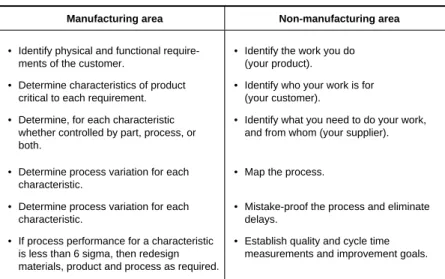
8. Case Studies of Six Sigma Improvement Projects 8.1 Manufacturing Applications: Microwave Oven Leakage . . . 165
8.2 Non-manufacturing Applications: Development of an Efficient Computerized Control System . . 172
8.3 R&D Applications: Design Optimization of Inner Shield of Omega CPT . . . 178
Appendices Table of Acronyms . . . 187
A-1 Standard Normal Distribution Table . . . 189
A-2 t-distribution Table of t(f;a) . . . 190
A-3 F-distribution Table of F(f1, f2;a) . . . 191
A-4 Control Limits for Various Control Charts . . . 195
A-5 GE Quality 2000: A Dream with a Great Plan . . 196
References . . . 200
Index . . . .203
This book has been written primarily for company managers and engineers in Asia who wish to grasp Six Sigma concepts, methodologies, and tools for quality and productivity promotion in their companies. However, this book will also be of interest to researchers, quality and productivity specialists, public sector employees, students and other professionals with an interest in quality management in general.
I have been actively involved over the last 20 years in indus- trial statistics and quality management teaching and consultation as a professor and as a private consultant. Six Sigma was recent- ly introduced into Korea around 1997, and I have found that Six Sigma is extremely effective for quality and productivity innova- tion in Korean companies. I have written two books on Six Sigma in Korean; one titled “The Theory and Practice of Six Sigma,” and the other called “Design for Six Sigma,” which are both best-sellers in Korea. In 2001, I had the honor of being invited to the “Symposium on Concept and Management of Six Sigma for Productivity Improvement” sponsored by the Asian Productivity Organization (APO) during 7–9 August as an invit- ed speaker. I met many practitioners from 15 Asian countries, and I was very much inspired and motivated by their enthusiasm and desire to learn Six Sigma. Subsequently, Dr. A.K.P. Mochtan, Program Officer of the Research & Planning Department, APO, came to me with an offer to write a book on Six Sigma as an APO publication. I gladly accepted his offer, because I wanted to share my experiences of Six Sigma with engineers and researchers in Asian countries, and I also desired a great improvement in quality and productivity in Asian countries to attain global competitiveness in the world market.
This book has three main streams. The first is to introduce an overview of Six Sigma, framework, and experiences (Chapters 1–3). The second is to explain Six Sigma tools, other manage- ment initiatives and some practical issues related to Six Sigma (Chapters 4–6). The third is to discuss practical questions in implementing Six Sigma and to present real case studies of
improvement projects (Chapters 7–8). This book can be used as a textbook or a guideline for a Champion or Master Black Belt course in Six Sigma training.
I would like to thank Dr. A.K.P. Mochtan and Director Yoshikuni Ohnishi of APO, who allowed me to write this book as an APO publication. I very much appreciate the assistance of Professor Moon W. Suh at North Carolina State University who examined the manuscript in detail and greatly improved the readability of the book. Great thanks should be given to Mr. Hui J. Park and Mr. Bong G. Park, two of my doctoral students, for undertaking the lengthy task of MS word processing of the man- uscript. I would especially like to thank Dr. Dag Kroslid, a Swedish Six Sigma consultant, for inspiring me to write this book and for valuable discussions on certain specific topics in the book.
Finally, I want to dedicate this book to God for giving me the necessary energy, health, and inspiration to finish the manuscript.
1.1 What is Six Sigma?
Sigma (σ) is a letter in the Greek alphabet that has become the statistical symbol and metric of process variation. The sigma scale of measure is perfectly correlated to such charac- teristics as defects-per-unit, parts-per-million defectives, and the probability of a failure. Six is the number of sigma mea- sured in a process, when the variation around the target is such that only 3.4 outputs out of one million are defects under the assumption that the process average may drift over the long term by as much as 1.5 standard deviations.
Six Sigma may be defined in several ways. Tomkins (1997) defines Six Sigma to be “a program aimed at the near-elimi- nation of defects from every product, process and transac- tion.” Harry (1998) defines Six Sigma to be “a strategic ini- tiative to boost profitability, increase market share and improve customer satisfaction through statistical tools that can lead to breakthrough quantum gains in quality.”
Six Sigma was launched by Motorola in 1987. It was the result of a series of changes in the quality area starting in the late 1970s, with ambitious ten-fold improvement drives. The top-level management along with CEO Robert Galvin devel- oped a concept called Six Sigma. After some internal pilot implementations, Galvin, in 1987, formulated the goal of
“achieving Six-Sigma capability by 1992” in a memo to all Motorola employees (Bhote, 1989). The results in terms of reduction in process variation were on-track and cost savings totalled US$13 billion and improvement in labor productivity achieved 204% increase over the period 1987–1997 (Losianowycz, 1999).
In the wake of successes at Motorola, some leading elec- tronic companies such as IBM, DEC, and Texas Instruments launched Six Sigma initiatives in early 1990s. However, it was
not until 1995 when GE and Allied Signal launched Six Sigma as strategic initiatives that a rapid dissemination took place in non-electronic industries all over the world (Hendricks and Kelbaugh, 1998). In early 1997, the Samsung and LG Groups in Korea began to introduce Six Sigma within their compa- nies. The results were amazingly good in those companies. For instance, Samsung SDI, which is a company under the Sam- sung Group, reported that the cost savings by Six Sigma pro- jects totalled US$150 million (Samsung SDI, 2000a). At the present time, the number of large companies applying Six Sigma in Korea is growing exponentially, with a strong verti- cal deployment into many small- and medium-size enterprises as well.
As a result of consulting experiences with Six Sigma in Korea, the author (Park et. al., 1999) believes that Six Sigma is a “new strategic paradigm of management innovation for com- pany survival in this 21st century, which implies three things:
statistical measurement, management strategy and quality cul- ture.” It tells us how good our products, services and process- es really are through statistical measurement of quality level. It is a new management strategy under leadership of top-level management to create quality innovation and total customer satisfaction. It is also a quality culture. It provides a means of doing things right the first time and to work smarter by using data information. It also provides an atmosphere for solving many CTQ (critical-to-quality) problems through team efforts.
CTQ could be a critical process/product result characteristic to quality, or a critical reason to quality characteristic. The for- mer is termed as CTQy, and the latter CTQx.
1.2 Why is Six Sigma Fascinating?
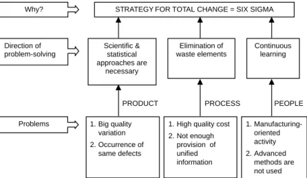
Six Sigma has become very popular throughout the whole world. There are several reasons for this popularity. First, it is regarded as a fresh quality management strategy which can replace TQC, TQM and others. In a sense, we can view the development process of Six Sigma as shown in Figure 1.1.
Many companies, which were not quite successful in imple- menting previous management strategies such as TQC and TQM, are eager to introduce Six Sigma.
Figure 1.1. Development process of Six Sigma in quality management Six Sigma is viewed as a systematic, scientific, statistical and smarter (4S) approach for management innovation which is quite suitable for use in a knowledge-based information society. The essence of Six Sigma is the integration of four ele- ments (customer, process, manpower and strategy) to provide management innovation as shown in Figure 1.2.
Figure 1.2. Essence of Six Sigma
Six Sigma provides a scientific and statistical basis for quali- ty assessment for all processes through measurement of quality levels. The Six Sigma method allows us to draw comparisons among all processes, and tells how good a process is. Through this information, top-level management learns what path to fol- low to achieve process innovation and customer satisfaction.
Second, Six Sigma provides efficient manpower cultivation and utilization. It employs a “belt system” in which the levels of mastery are classified as green belt, black belt, master black belt and champion. As a person in a company obtains certain
Customer Process Manpower
Strategy
Management innovation Systematic and
Scientific Approach Six Sigma
QC SQC TQC TQM Six Sigma
ISO 9000 Series
Scientific management tools such as SPC, TPM,
QE and TCS
training, he acquires a belt. Usually, a black belt is the leader of a project team and several green belts work together for the project team.
Third, there are many success stories of Six Sigma appli- cation in well known world-class companies. As mentioned earlier, Six Sigma was pioneered by Motorola and launched as a strategic initiative in 1987. Since then, and particular- ly from 1995, an exponentially growing number of presti- gious global firms have launched a Six Sigma program. It has been noted that many globally leading companies run Six Sigma programs (see Figure 3), and it has been well known that Motorola, GE, Allied Signal, IBM, DEC, Texas Instruments, Sony, Kodak, Nokia, and Philips Electronics among others have been quite successful in Six Sigma. In Korea, the Samsung, LG, Hyundai groups and Korea Heavy Industries & Construction Company have been quite suc- cessful with Six Sigma.
Lastly, Six Sigma provides flexibility in the new millennium of 3Cs, which are:
• Change: Changing society
• Customer: Power is shifted to customer and customer demand is high
• Competition: Competition in quality and productivity The pace of change during the last decade has been unprece- dented, and the speed of change in this new millennium is per- haps faster than ever before. Most notably, the power has shift- ed from producer to customer. The producer-oriented industri- al society is over, and the customer-oriented information soci- ety has arrived. The customer has all the rights to order, select and buy goods and services. Especially, in e-business, the cus- tomer has all-mighty power. Competition in quality and pro- ductivity has been ever-increasing. Second-rate quality goods cannot survive anymore in the market. Six Sigma with its 4S (systematic, scientific, statistical and smarter) approaches pro- vides flexibility in managing a business unit.
1.3 Key Concepts of Management
The core objective of Six Sigma is to improve the perfor- mance of processes. By improving processes, it attempts to achieve three things: the first is to reduce costs, the second is to improve customer satisfaction, and the third is to increase revenue, thereby, increasing profits.
Figure 1.3. Globally well known Six Sigma companies
1.3.1 Process
A general definition of a process is an activity or series of activities transforming inputs to outputs in a repetitive flow as shown in Figure 1.4. For companies, the output is predomi- nantly a product taking the form of hardware goods with their associated services. However, an R&D activity or a non- manufacturing service activity which does not have any form of hardware goods could also be a process.
Figure 1.4. The process with inputs and outputs
Input variables (control factors)
Input variables (noise factors)
Process Process characteristics
X 1 X 2 X 3 X n
V 1 V 2 V 3 V n
…
…
Output, Y Product characteristics
1987 1989 1991 1993 1995 1997 1999
American Express Johnson & Johnson Samsung Group LG Group Ericsson NCR Nokia Philips Solectron US Postal Service Dow Chemical
DuPont NEC Samsung SDI LG Electronics Sony Toshiba Whirlpool GE
Allied Signal TI
ABB Kodak DEC IBM Motorola
Literally, the inputs can be anything from labor, materials, machines, decisions, information and measurements to tem- perature, humidity and weight. Inputs are either control fac- tors which can be physically controlled, or noise factors which are considered to be uncontrollable, too costly to control, or not desirable to control.
The model of Six Sigma in terms of processes and improve- ment is that yis a function of xand v:
y = f(x1, x2, ..., xk; v1, v2, ..., vm)
Here, yrepresents the result variable (characteristics of the process or product), xrepresents one or more control factors, and vrepresents one or more noise factors. The message in the process is to find the optimal levels of x variables which give desired values of yas well as being robust to the noise factors v. The word “robust” means that the yvalues are not changed much as the levels of noise factors are changed.
Any given process will have one or more characteristics specified against which data can be collected. These charac- teristics are used for measuring process performance. To mea- sure the process performance, we need data for the relevant characteristics. There are two types of characteristics: contin- uous and discrete. Continuous characteristics may take any measured value on a continuous scale, providing continuous data, whereas discrete characteristics are based on counts, providing attribute data. Examples of continuous data are thickness, time, speed and temperature. Typical attribute data are counts of pass/fail, acceptable/unacceptable, good/bad or imperfections.
1.3.2 Variation
The data values for any process or product characteristic always vary. No two products or characteristics are exactly alike because any process contains many sources of vari- ability. The differences among products may be large, or they may be immeasurably small, but they are always pre- sent. The variation, if the data values are measured, can be
visualized and statistically analyzed by means of a distribu- tion that best fits the observations. This distribution can be characterized by:
• Location (average value)
• Spread (span of values from smallest to largest)
• Shape (the pattern of variation – whether it is symmet- rical, skewed, etc.)
Variation is indeed the number one enemy of quality con- trol. It constitutes a major cause of defectives as well as excess costs in every company. Six Sigma, through its tracking of process performance and formalized improvement methodol- ogy, focuses on pragmatic solutions for reducing variation.
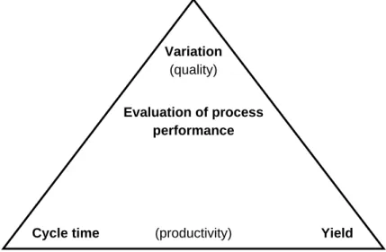
Variation is the key element of the process performance trian- gle as shown in Figure 1.5. Variation, which is the most important, relates to “how close are the measured values to the target value,” cycle time to “how fast” and yield to “how much.” Cycle time and yield are the two major elements of productivity.
Figure 1.5. Process performance triangle Variation
(quality)
Evaluation of process performance
Cycle time (productivity) Yield
There are many sources of variation for process and prod- uct characteristics. It is common to classify them into two types: common causes and special causes. Common causes refer to the sources of variation within a process that have a stable and repeatable distribution over time. This is called “in a state of statistical control.” The random variation, which is inherent in the process, is not easily removable unless we change the very design of the process or product, and is a common cause found everywhere. Common causes behave like a stable system of chance causes. If only common causes of variation are present and do not change, the output of a process is predictable as shown in Figure 1.6.
Figure 1.6. Variation: Common and special causes
Special causes (often called assignable causes) refer to any factors causing variation that are usually not present in the
If only common causes of variation are present, the output of a process forms a distribution that is stable over time and is predictable:
If special causes of variation are present, the process output is not stable over time:
SIZE
TIME
PREDICTION TARGET
LINE
SIZE
TIME
PREDICTION TARGET
LINE
process. That is, when they occur, they make a change in the process distribution. Unless all the special causes of variation are identified and acted upon, they will continue to affect the process output in unpredictable ways. If special causes are present, the process output is not stable over time.
1.3.3 Cycle time, yield and productivity
Every process has a cycle time and yield. The cycle time of a process is the average time required for a single unit to com- plete the transformation of all input factors into an output.
The yield of a process is the amount of output related to input time and pieces. A more efficient transformation of input fac- tors into products will inevitably give a better yield.
Productivity is used in many different aspects (see Toru Sase (2001)). National productivity can be expressed as GDP/population where GDP means the gross domestic prod- uct. Company productivity is generally defined as the “func- tion of the output performance of the individual firm com- pared with its input.” Productivity for industrial activity has been defined in many ways, but the following definition pro- posed by the European Productivity Agency (EPA) in 1958 is perhaps the best.
• Productivity is the degree of effective utilization of each element of production.
• Productivity is, above all, an attitude of mind. It is based on the conviction that one can do things better today than yesterday, and better tomorrow than today.
It requires never-ending efforts to adapt economic activ- ities to changing conditions, and the application of new theories and methods. It is a firm belief in the progress of human beings.
The first paragraph refers to the utilization of production elements, while the second paragraph explains the social effects of productivity. Although the product is the main out- put of an enterprise, other tasks such as R&D activities, sale of products and other service activities are also closely linked
to productivity. In economic terms, productivity refers to the extent to which a firm is able to optimize its management resources in order to achieve its goals. However, in this book we adopt the definition of productivity as in the first para- graph, which is narrow in scope. Thus, if cycle time and yield in the process performance triangle of Figure 1.5 are improved, productivity can be improved accordingly.
1.3.4 Customer satisfaction
Customer satisfaction is one of the watchwords for compa- ny survival in this new 21st century. Customer satisfaction can be achieved when all the customer requirements are met. Six Sigma emphasizes that the customer requirements must be ful- filled by measuring and improving processes and products, and CTQ (critical-to-quality) characteristics are measured on a con- sistent basis to produce few defects in the eyes of the customer.
The identification of customer requirements is ingrained in Six Sigma and extended into the activity of translating require- ments into important process and product characteristics. As customers rarely express their views on process and product characteristics directly, a method called QFD (quality function deployment) is applied for a systematic translation (see Chap- ter 4). Using QFD, it is possible to prioritize the importance of each characteristic based on input from the customer.
Having identified the CTQ requirements, the customer is usually asked to specify what the desired value for the char- acteristic is, i.e., target value, and what a defect for the char- acteristic is, i.e., specification limits. This vital information is utilized in Six Sigma as a basis for measuring the performance of processes.
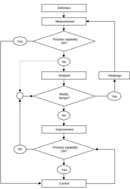
Six Sigma improvement projects are supposed to focus on improvement of customer satisfaction which eventually gives increased market share and revenue growth. As a result of rev- enue growth and cost reduction, the profit increases and the commitment to the methodology and further improvement projects are generated throughout the company. This kind of
loop is called “Six Sigma loop of improvement projects,” and was suggested by Magnusson, et. al. (2001). This loop is shown in Figure 1.7.
Figure 1.7. Six Sigma loop of improvement projects
1.4 Measurement of Process Performance
Among the dimensions of the process performance triangle in Figure 1.5, variation is the preferred measurement for process performance in Six Sigma. Cycle time and yield could have been used, but they can be covered through variation.
For example, if a cycle time has been specified for a process, the variation of the cycle time around its target value will indi- cate the performance of the process in terms of this character- istic. The same applies to yield.
The distribution of a characteristic in Six Sigma is usually assumed to be Normal (or Gaussian) for continuous variables, and Poissonian for discrete variables. The two parameters that determine a Normal distribution are population mean, µ, and population standard deviation, σ. The mean indicates the loca- tion of the distribution on a continuous scale, whereas the standard deviation indicates the dispersion.
Variation
Cycle time Yield
Improvement project
Commitment Cost
Profit
Customer satisfaction
Market share
Revenue
1.4.1 Standard deviation and Normal distribution
The population parameters, µ (population mean), σ (popu- lation standard deviation) and σ2 (population variance), are usually unknown, and they are estimated by the sample sta- tistics as follows.
–y= sample mean = estimate of µ
s= sample standard deviation = estimate of σ V = sample variance = estimate of σ2
If we have a sample of size nand the characteristics are y1,y2, ..., yn, then µ, σ and σ2 are estimated by, respectively
However, if we use an –x– R control chart, in which there are ksubgroups of size n, σ can be estimated by
where –
R = Ri/ n, and Riis the range for each subgroup and d2 is a constant value that depends on the sample size n. The val- ues of d2 can be found in Appendix A-4.
Many continuous random variables, such as the dimension of a part and the time to fill the order for a customer, follow a normal distribution.
Figure 1.8 illustrates the characteristic bell shape of a nor- mal distribution where X is the normal random variable, uis the population mean and σ is the population standard devia- tion. The probability density function (PDF), f(x), of a normal distribution is
d2
s= R (1.2)
n y y
y y + + + n
= 1 2 …
V
Σ
s = (1.1)
1 ) (
1
2
– –
= = n
y y V
n
i i
where we usually denote X ~ N(µ, σ2)
When X ~ N(µ, σ2), it can be converted into standard normal variable Z ~ N(0,1) using the relationship of variable trans- formation,
whose probability density function is
Figure 1.8. Normal distribution
Area = 0.6826894
Area = 0.9544998
Area = 0.9973002
µ – 3σ µ – 2σ µ – σ µ µ + σ µ + 2σ µ + 3σ
2
2 1
2 ) 1
(z e z
f = − (1.5)
= X −
Z (1.4)
2
2 1
2 ) 1 (
− −
=
x
e x
f (1.3)
1.4.2 Defect rate, ppm and DPMO
The defect rate, denoted by p, is the ratio of the number of defective items which are out of specification to the total num- ber of items processed (or inspected). Defect rate or fraction of defective items has been used in industry for a long time. The number of defective items out of one million inspected items is called the ppm (parts-per-million) defect rate. Sometimes a ppm defect rate cannot be properly used, in particular, in the cases of service work. In this case, a DPMO (defects per mil- lion opportunities) is often used. DPMO is the number of defective opportunities which do not meet the required specifi- cation out of one million possible opportunities.
1.4.3 Sigma quality level
Specification limits are the tolerances or performance ranges that customers demand of the products or processes they are purchasing. Figure 1.8 illustrates specification limits as the two major vertical lines in the figure. In the figure, LSL means the lower specification limit, USL means the upper specification limit and T means the target value. The sigma quality level (in short, sigma level) is the distance from the process mean (µ) to the closer specification limit.
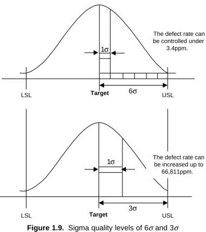
In practice, we desire that the process mean to be kept at the target value. However, the process mean during one time period is usually different from that of another time period for various reasons. This means that the process mean constantly shifts around the target value. To address typical maximum shifts of the process mean, Motorola added the shift value
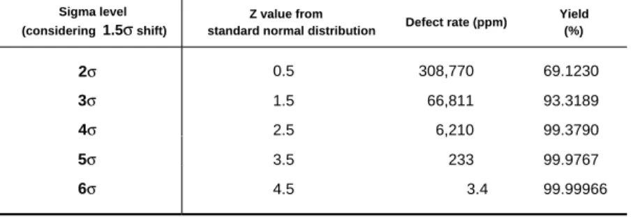
±1.5σ to the process mean. This shift of the mean is used when computing a process sigma level as shown in Figure 1.10. From this figure, we note that a 6σ quality level corre- sponds to a 3.4ppm rate. Table 1.1 illustrates how sigma qual- ity levels would equate to other defect rates and organization- al performances. Table 1.2 shows the details of this relation- ship when the process mean is ±1.5σ shifted.
Figure 1.9. Sigma quality levels of 6σand 3σ
Figure 1.10. Effects of a 1.5σshift of process mean when 6σquality level is achieved 6
– +6 –7.5 +4.5
0.001 ppm
0.001
ppm 0 ppm 3.4 ppm
Target USL
6 +
LSL 5 . 7 –
USL 5 . 4 + Target
5 . 1 – LSL
6 –
LSL USL
6σ 1σ
The defect rate can be controlled under
3.4ppm.
3σ
1σ The defect rate can
be increased up to 66,811ppm.
Target
Target
USL LSL
Table 1.1. ppm changes when sigma quality level changes
1.4.4 DPU, DPO and Poisson distribution
Let us suppose for the sake of discussion that a certain prod- uct design may be represented by the area of a rectangle. Let us also postulate that each rectangle contains eight equal areas of opportunity for non-conformance (defect) to standard. Figure 1.11 illustrates three particular products. The first one has one defect and the third one has two defects.
Figure 1.11. Products consisting of eight equal areas of opportunity for non-conformance The defects per unit (DPU)is defined as
In Figure 1.11, DPU is 3/3 = 1.00, which means that, on average, each unit product will contain one such defect. Of course, this assumes that the defects are randomly distributed.
Total number of unit products produced Total defects observed of number
=
DPU (1.6)
Product 1 Product 2 Product 3
Sigma quality Process mean, fixed Process mean, with 1.5σ shift level Non-defect Defect rate Non-defect Defect rate
rate (%) (ppm) rate (%) (ppm)
σ 68.26894 317,311.000 30.2328 697,672.0
2σ 95.44998 45,500.000 69.1230 308,770.0
3σ 4σ 5σ 6σ
99.73002 2,700.000 93.3189 66,811.0
99.99366 63.400 99.3790 6,210.0
99.999943 0.570 99.97674 233.0
99.9999998 0.002 99.99966 3.4
We must also recognize, however, that within each unit of product there are eight equal areas of opportunity for non- conformance to standard.
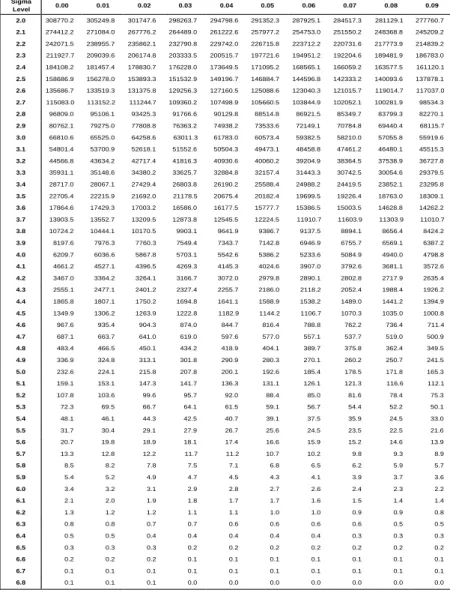
Table 1.2. Detailed conversion between ppm (or DPMO) and sigma quality level when the process mean is ±1.5σshifted
Sigma
Level 0.00 0.01 0.02 0.03 0.04 0.05 0.06 0.07 0.08 0.09
2.0 308770.2 305249.8 301747.6 298263.7 294798.6 291352.3 287925.1 284517.3 281129.1 277760.7 2.1 274412.2 271084.0 267776.2 264489.0 261222.6 257977.2 254753.0 251550.2 248368.8 245209.2 2.2 242071.5 238955.7 235862.1 232790.8 229742.0 226715.8 223712.2 220731.6 217773.9 214839.2 2.3 211927.7 209039.6 206174.8 203333.5 200515.7 197721.6 194951.2 192204.6 189481.9 186783.0 2.4 184108.2 181457.4 178830.7 176228.0 173649.5 171095.2 168565.1 166059.2 163577.5 161120.1 2.5 158686.9 156278.0 153893.3 151532.9 149196.7 146884.7 144596.8 142333.2 140093.6 137878.1 2.6 135686.7 133519.3 131375.8 129256.3 127160.5 125088.6 123040.3 121015.7 119014.7 117037.0 2.7 115083.0 113152.2 111244.7 109360.2 107498.9 105660.5 103844.9 102052.1 100281.9 98534.3 2.8 96809.0 95106.1 93425.3 91766.6 90129.8 88514.8 86921.5 85349.7 83799.3 82270.1 2.9 80762.1 79275.0 77808.8 76363.2 74938.2 73533.6 72149.1 70784.8 69440.4 68115.7 3.0 66810.6 65525.0 64258.6 63011.3 61783.0 60573.4 59382.5 58210.0 57055.8 55919.6 3.1 54801.4 53700.9 52618.1 51552.6 50504.3 49473.1 48458.8 47461.2 46480.1 45515.3 3.2 44566.8 43634.2 42717.4 41816.3 40930.6 40060.2 39204.9 38364.5 37538.9 36727.8 3.3 35931.1 35148.6 34380.2 33625.7 32884.8 32157.4 31443.3 30742.5 30054.6 29379.5 3.4 28717.0 28067.1 27429.4 26803.8 26190.2 25588.4 24988.2 24419.5 23852.1 23295.8 3.5 22705.4 22215.9 21692.0 21178.5 20675.4 20182.4 19699.5 19226.4 18763.0 18309.1 3.6 17864.6 17429.3 17003.2 16586.0 16177.5 15777.7 15386.5 15003.5 14628.8 14262.2 3.7 13903.5 13552.7 13209.5 12873.8 12545.5 12224.5 11910.7 11603.9 11303.9 11010.7
3.8 10724.2 10444.1 10170.5 9903.1 9641.9 9386.7 9137.5 8894.1 8656.4 8424.2
3.9 8197.6 7976.3 7760.3 7549.4 7343.7 7142.8 6946.9 6755.7 6569.1 6387.2
4.0 6209.7 6036.6 5867.8 5703.1 5542.6 5386.2 5233.6 5084.9 4940.0 4798.8
4.1 4661.2 4527.1 4396.5 4269.3 4145.3 4024.6 3907.0 3792.6 3681.1 3572.6
4.2 3467.0 3364.2 3264.1 3166.7 3072.0 2979.8 2890.1 2802.8 2717.9 2635.4
4.3 2555.1 2477.1 2401.2 2327.4 2255.7 2186.0 2118.2 2052.4 1988.4 1926.2
4.4 1865.8 1807.1 1750.2 1694.8 1641.1 1588.9 1538.2 1489.0 1441.2 1394.9
4.5 1349.9 1306.2 1263.9 1222.8 1182.9 1144.2 1106.7 1070.3 1035.0 1000.8
4.6 967.6 935.4 904.3 874.0 844.7 816.4 788.8 762.2 736.4 711.4
4.7 687.1 663.7 641.0 619.0 597.6 577.0 557.1 537.7 519.0 500.9
4.8 483.4 466.5 450.1 434.2 418.9 404.1 389.7 375.8 362.4 349.5
4.9 336.9 324.8 313.1 301.8 290.9 280.3 270.1 260.2 250.7 241.5
5.0 232.6 224.1 215.8 207.8 200.1 192.6 185.4 178.5 171.8 165.3
5.1 159.1 153.1 147.3 141.7 136.3 131.1 126.1 121.3 116.6 112.1
5.2 107.8 103.6 99.6 95.7 92.0 88.4 85.0 81.6 78.4 75.3
5.3 72.3 69.5 66.7 64.1 61.5 59.1 56.7 54.4 52.2 50.1
5.4 48.1 46.1 44.3 42.5 40.7 39.1 37.5 35.9 24.5 33.0
5.5 31.7 30.4 29.1 27.9 26.7 25.6 24.5 23.5 22.5 21.6
5.6 20.7 19.8 18.9 18.1 17.4 16.6 15.9 15.2 14.6 13.9
5.7 13.3 12.8 12.2 11.7 11.2 10.7 10.2 9.8 9.3 8.9
5.8 8.5 8.2 7.8 7.5 7.1 6.8 6.5 6.2 5.9 5.7
5.9 5.4 5.2 4.9 4.7 4.5 4.3 4.1 3.9 3.7 3.6
6.0 3.4 3.2 3.1 2.9 2.8 2.7 2.6 2.4 2.3 2.2
6.1 2.1 2.0 1.9 1.8 1.7 1.7 1.6 1.5 1.4 1.4
6.2 1.3 1.2 1.2 1.1 1.1 1.0 1.0 0.9 0.9 0.8
6.3 0.8 0.8 0.7 0.7 0.6 0.6 0.6 0.6 0.5 0.5
6.4 0.5 0.5 0.4 0.4 0.4 0.4 0.4 0.3 0.3 0.3
6.5 0.3 0.3 0.3 0.2 0.2 0.2 0.2 0.2 0.2 0.2
6.6 0.2 0.2 0.2 0.1 0.1 0.1 0.1 0.1 0.1 0.1
6.7 0.1 0.1 0.1 0.1 0.1 0.1 0.1 0.1 0.1 0.1
6.8 0.1 0.1 0.1 0.0 0.0 0.0 0.0 0.0 0.0 0.0
Because of this, we may calculate the defects per unit oppor- tunity (DPO)
where mis the number of independent opportunities for non- conformance per unit. In the instance of our illustrated exam- ple, since m= 8,
or 12.5 percent. Inversely, we may argue that there is an 84 percent chance of not encountering a defect with respect to any given unit area of opportunity. By the same token, the defects-per- million opportunities (DPMO) becomes
It is interesting to note that the probability of zero defects, for any given unit of product, would be (0.875)8= 0.3436, or 34.36 percent. Then, we may now ask the question, “What is the probability that any given unit of product will contain one, two or three more defects?” This question can be answered by applying a Poisson distribution.
The probability of observing exactly X defects for any given unit of product is given by the Poisson probability den- sity function:
where e is a constant equal to 2.71828 and λis the average num- ber of defects for a unit of product. To better relate the Poisson relation to our example, we may rewrite the above equation as
! ) ) (
( x
DPU x e
p
x
−DPU
= , (1.9)
,… 3 , 2 , 1 , 0
! , ) ( )
( = = = − x=
x x e p x X P
x
(1.8) 000 . , 125 000 , 000 , 8 1 00 . 000 1 , 000 ,
1 = =
× ×
= m DPMO DPU
125 . 8 0 1.00 =
= DPO
m
DPO= DPU (1.7)
which can be effectively used when DPO = DPU / m is less than 10 percent and m is relatively large. Therefore, the prob- ability that any given unit of product will contain only one defect is
For the special case of x= 0, which is the case of zero defect for a given unit of product, the probability becomes
and this is somewhat different from the probability 0.3436 that was previously obtained. This is because DPOis greater than 10 percent and m is rather small.
1.4.5 Binomial trials and their approximations
A binomial distribution is useful when there are only two results (e.g., defect or non-defect, conformance or non-con- formance, pass or fail) which is often called a binomial trial.
The probability of exactly x defects in n inspected trials whether they are defects or not, with probability of defect equal to pis
where q = 1 – pis the probability of non-defect. In practice, the computation of the probability P(a≤ X≤b) is usually dif- ficult if nis large. However, if np ≥ 5 and nq≥ 5, the proba- bility can be easily approximated by using E(X)= µ= np and V(X) = σ2= npq, where Eand Vrepresent expected value and variance, respectively.
if p≤ 0.1 and n≥ 50, the probability in (1.10) can be well approximated by a Poisson distribution as follows.
! ) ) (
( x
np x e
p
x
−np
= . (1.11)
n, x
q x p n x q n x p x n p x X
p x nx x n x, 0,1,2, , )!
(
! ) !
( )
( = …
= −
=
=
= − −
(1.10)
3679 . 0 )
(x =e−1.00 = p
3679 .
! 0 1
) 00 . 1 ) (
(
1 00 .
1 =
= e− x
p .
Hence, for the case of Figure 1.11, the probability of zero defects for a given unit of product can be obtained by either (1.10) or (1.11).
Note that since p= 0.125 is not smaller than 0.1 and n= 8 is not large enough, the Poisson approximation from (1.11) is not good enough.
1.4.6 Process capability index
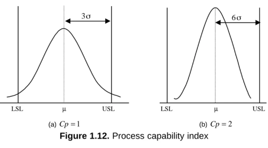
There are two metrics that are used to measure the process capability. One is potential process capability index (Cp), and another is process capability index (Cpk)
(1) Potential process capability index (Cp)
Cpindex is defined as the ratio of specification width over the process spread as follows.
The specification width is predefined and fixed. The process spread is the sole influence on the Cp index. The population standard deviation, σ, is usually estimated by the equations (1.1) or (1.2). When the spread is wide (more variation), the Cp value is small, indicating a low process capability. When the spread is narrow (less variation), the Cp value becomes larger, indicating better process capability.
USL – LSL
Cp processspread 6
ion width specificat
=
= (1.12)
Since n=8, p=DPO=0.125, q=0.875, np=8 1.125=1 and x=0, from (1.10), (0.125) (0.875) 0.3436
! 8
! 0
! ) 8 0
(x= = 0 8 =
p ,
from (1.11), 0.3679
! 0
) 1 ) ( 0 (
0 1
=
=
= e− x
p .
×
Figure 1.12. Process capability index
The Cp index does not account for any process shift. It assumes the ideal state when the process is at the desirable tar- get, centered exactly between the two specification limits.
(2) Process capability index (Cpk)
In real life, very few processes are at their desirable target.
An off-target process should be “penalized” for shifting from where it should be. Cpk is the index for measuring this real capability when the off-target penalty is taken into considera- tion. The penalty, or degree of bias, kis defined as:
and the process capability index is defined as:
When the process is perfectly on target, k= 0 and Cpk= Cp.
Note that Cpkindex inc-reases as both of the following con- ditions are satisfied.
• The process is as close to the target as possible (kis small).
• The process spread is as small as possible (process vari- ation is small).
) 1
( k
Cp
Cpk = − . (1.14)
(USL – LSL) k T
2 1
) mean(
process –
) target(
= (1.13)
(a) Cp=1 (b) Cp=2
LSL µ USL LSL µ USL
3 6
Figure 1.13. Process capability index (Cpk)
We have dealt with the case when there are two specifica- tion limits, USLand LSL. However, when there is a one-sided specification limit, or when the target is not specified, Cpk may be more conveniently calculated as:
We often use upper capability index (CPU) and lower capabili- ty index (CPL). CPU is the upper tolerance spread divided by the actual upper process spread. CPLis defined as the lower tol- erance spread divided by the actual lower process spread.
Cpkin (1.15) may be defined as the minimum of CPUor CPL.
It relates the scaled distance between the process mean and the closest specification limit to half the total process spread.
(3) Relationship between Cp, Cpkand Sigma level
If the process mean is centered, that is µ = T, and USL – LSL = 6σ, then from (1.12), it is easy to know that Cp = 1, and the distance from µto the specification limit is 3σ. In this
) , min(CPU CPL
Cpk = (1.17)
3
=USL−
CPU ,
3
CPL= −LSL (1.16)
3
from limit ion specificat closer
- ) mean(
process
=
Cpk . (1.15)
) 6 1
( USL LSL
k
Cpk= − − ,
bias of degree
2
=
−
= −
LSL USL k T
LSL T µ USL
case, the sigma (quality) level becomes 3σ, and the relation- ship between Cp and the sigma level is
However, in the long run the process mean could shift at most by 1.5σ to the right or left hand side, and the process mean cannot be centered, that is, it can be biased.
In the long-term, if the process mean is 1.5σ biased and Cpk
= 1 then the sigma level becomes 3σ + 1.5σ = 4.5σ. Figure 1.14 shows a 6σ process with typical 1.5σ shift. In this case, Cpk = 1.5 and the sigma level is 6σ. In general, the relation- ship between Cpkand the sigma level is
Hence, in the long-term the relationship between Cpand Cpk is from (1.18) and (1.19),
Table 1.3 shows the relationship between process capability index and sigma level.
Table 1.3 Relationship between Cp, Cpkand Sigma level Cp Cpk (5.1σ shift is allowed) Quality level
0.50 0.00 1.5σ
0.67 0.17 2.0σ
0.83 0.33 2.5σ
1.00 0.50 3.0σ
1.17 0.67 3.5σ
1.33 0.83 4.0σ
1.50 1.00 4.5σ
1.67 1.17 5.0σ
1.83 1.33 5.5σ
2.00 1.50 6.0σ
5 .
−0
=Cp
Cpk . (1.20)
5 . 1 3
level
Sigma = ×Cpk+
) 5 . 0 (
3× +
= Cpk (1.19)
×Cp
=3 level
Sigma (1.18)
1.4.7 Rolled throughput yield (RTY)
Rolled throughput yield (RTY) is the final cumulative yield when there are several processes connected in series. RTY is the amount of non-defective products produced in the final process compared with the total input in the first process.
Figure 1.14 RTY and yield of each process
For example, as shown in Figure 1.14, there are four processes (A, B, C and D) connected in consecutive series, and each process has a 90% yield.
Then RTY of these processes is RTY = 0.9 × 0.9 × 0.9 ×0.9 = 0.656.
If there are kprocesses in series, and the ith process has its own yield yi, then RTY of these kprocesses is
1.4.8 Unified quality level for multi-characteristics
In reality, there is more than one characteristic and we are faced with having to compute a unified quality level for multi- characteristics. As shown in Table 1.4, suppose there are three characteristics and associated defects. Table 1.4 illustrates how to compute DPU, DPO, DPMO and sigma level. The way to convert from DPMO (or ppm) to sigma level can be found in Table 1.2.
yk
× ×y ×
= y1 2 …
RTY (1.21)
Process
Yield
A B C D
90% 90% 90% 90%
RTY
65.6%
Table 1.4. Computation of unified quality level
1.4.9 Sigma level for discrete data
When a given set of data is continuous, we can easily obtain the mean and standard deviation. Also from the given specification limits, we can compute the sigma level. Howev- er, if the given set of data is discrete, such as number of defects, we should convert the data to yield and obtain the sigma level using the standard normal distribution in Appen- dix table A-1. Suppose the non-defect rate for a given set of discrete data is y. Then the sigma level Z can be obtained from the relationship Φ(z) = y, where Φ is the standard cumulative normal distribution
For example, if y= 0.0228, then z= 2.0 from Appendix A-1.
If this y value is obtained in the long-term, then a short-term sigma level should be
considering the 1.5σmean shift. Here, Zsand Zlmean a short- term and long-term sigma level, respectively.
The methods of computing sigma levels are explained below for each particular case.
5 . +1
= l
s Z
Z , (1.23)
y
dw e
z z
w
=
= Φ −∞
−
2 ) 1
( 2
2
(1.22)
∫
Characteristic number
Number of defects
Number of units
Opportunities per unit
Total
opportunities DPU DPO DPMO Sigmalevel
1 2 3
78 29 64
600 241 180
10 100 3
6,000 24,100 540
0.130 0.120 0.356
0.0130 0.0012 0.1187
13,000 1,200 118,700
3.59 4.55 2.59
Total 171 30,640 0.00558 5,580 3.09
(1) Case of DPU
Suppose that the pinhole defects in a coating process have been found in five units out of 500 units inspected from a long-term investigation. Since the number of defects follows a Poisson distribution, and DPU = 5/500 = 0.01, the probabili- ty of zero defect is from (1.9),
and the corresponding Z value is Z = 2.33. Since the set of data has been obtained for a long-term, the short-term sigma level is Zs= 2.33 + 1.5 = 3.83
(2) Case of defect rate
If r products, whose measured quality characteristics are outside the specifications, have been classified to be defective out of n products investigated, the defect rate is p= r/n, and the yield is y= 1 – p. Then we can find the sigma level Zfrom the relationship (1.22). For example, suppose two products out of 100 products have a quality characteristic which is out- side of specification limits. Then the defect rate is 2 percent, and the yield is 98 percent. Then the sigma level is approxi- mately Z = 2.05 from (1.22).
If this result is based on a long-term investigation, then the short-term sigma level is Zs = 2.05 + 1.5 = 3.55.
Table 1.5 shows the relationship between short-term sigma level, Zvalue, defect rate and yield.
Table 1.5. Relationship between sigma level, defect rate and yield
Sigma level
(considering 1.5σ shift) Z value from
standard normal distribution Defect rate (ppm) Yield (%)
2σ 0.5 308,770 69.1230
3σ 1.5 66,811 93.3189
4σ 2.5 6,210 99.3790
5σ 3.5 233 99.9767
6σ 4.5 3.4 99.99966
99005 .
01 0
.
0 =
=
=e− e−
y DPU ,
(3) Case of RTY
Suppose there are three processes in consecutive series, and the yield of each process is 0.98, 0.95, and 0.96, respectively.
Then RTY = 0.98 × 0.95 ×0.96 = 0.89376, and the sigma lev- els of the processes are 3.55, 3.14, and 3.25, respectively. How- ever, the sigma level of the entire process turns out to be 2.75, which is much lower than that of each process.
1.5 Relationship between Quality and Productivity
Why should an organization try to improve quality and productivity? If a firm wants to increase its profits, it should increase productivity as well as quality. The simple idea that increasing productivity will increase profits may not always be right. The following example illustrates the folly of such an idea.
Suppose Company A has produced 100 widgets per hour, of which 10 percent are defective for the past 3 years. The Board of Directors demands that top-level management increase productivity by 10 percent. The directive goes out to the employees, who are told that instead of producing 100 widgets per hour, the company must produce 110. The responsibility for producing more widgets falls on the employ- ees, creating stress, frustration, and fear. They try to meet the new demand but must cut corners to do so. The pressure to raise productivity creates a defect rate of 20 percent and increases good production to only 88 units, fewer than the original 90 as shown in Table 1.6 (a). This indicates that pro- ductivity increase is only meaningful when the level of quality does not deteriorate.
Very often, quality improvement results in a productivity improvement. Let’s take an example. Company B produces 100 widgets per hour with 10% defectives. The top-level man- agement is continually trying to improve quality, thereby increasing the productivity. Top-level management realizes that the company is making 10% defective units, which trans- lates into 10% of the total cost being spent in making bad