Smithsonian Contributions to Astrophysics

(1)

Smithsonian

Contributions to Astrophysics

VOLUME 2, NUMBER 5

GEOMAGNETISM AND THE EMISSION-LINE CORONA, 1950-1953

By BARBARA BELL and HAROLD GLAZER

SMITHSONIAN INSnTUTION

Washington, D. C.

1957

For sale by the Superintendent of Documents, U. S. Government Printing Office Washington 25, D. C. - Price 65 cents

(2)

Publications of the Astrophysical Observatory

This series, Smithsonian Contributions to Astrophysics, was inaugurated in 1956 to provide a proper communication for the results of research con- ducted at the Astrophysical Observatory of the Smithsonian Institution.

Its purpose is the "increase and diffusion of knowledge" in the field of astro- physics, with particular emphasis on problems of the sun, the earth, and the solar system. Its pages are open to a limited number of papers by other investigators with whom we have common interests.

Another series is Annals of the Astrophysical Observatory. It was started in 1900 by the Observatory's first director, Samuel P. Langley, and has been published about every 10 years since that date. These quarto volumes, some of which are still available, record the history of the Observatory's researches and activities.

Many technical papers and volumes emanating from the Astrophysica Observatory have appeared in the Smithsonian Miscellaneous Collections.

Among these are Smithsonian Physical Tables, Smithsonian Meteorological Tables, and World Weather Records.

Additional information concerning these publications may be secured from the Editorial and Publications Division, Smithsonian Institution Washington, D. C.

FRED L. WHIPPLB, Director,

Astrophysical Observatory, Smithsonian Institution.

Cambridge, Mass.

(3)

Page Introduction 51 Part I. Single intensity index for each coronal line 57 Green line, X5303 58 Correlation coefficient . 62 Red line, X6374 62 Red and green lines, simultaneously 63 Yellow line, X5694 64 Green line intensity around zero-days defined by large Kp . . 65 Heliographic latitude of the earth 66 Active centers 66 M-regions 67 Summary 69 Part II. Separate intensity indices for northern and for southern

solar hemispheres 69 Green line 70 Hemisphere versus angular distance 79 Red line 88 Red and green lines, simultaneously 91 Yellow line 91 Part III. Inverse solutions for hemisphere effects 91 M-regions 93 Other periods: 1942-44, 1944-49 97 Yellow line 102 Summary and interpretation 103 Acknowledgments 105 References 106 Abstract 107

m

(4)

(5)

Geomagnetism and the Emission-Line Corona, 1950-1953

By Barbara Bell1 and Harold Glazer

I ntroduction

In this paper we investigate the relation between the intensity of the coronal emission- lines, X5303 and X6374, and the geomagnetic character figure, Kp, generally interpreted as a measure of the solar corpuscular radiation.

However, a summary of previous research on the general problem of solar-geomagnetic relations may be useful. We are limiting this summary to those effects generally thought to arise from solar corpuscular radiation; and we are not considering geomagnetic phenomena believed to arise from solar ultraviolet radiation.

The displaced and greatly broadened Balmer lines observed independently by Meinel (1951) and Gartlein (1950, 1951) in spectra of aurorae comprise the only direct evidence for streams of corpuscles striking the earth. Spectra obtained by Meinel during the intense aurora of Aug. 18 and 19, 1950, indicated a velocity of impact above 3000 km/sec for the protons. If the corpuscles come directly from the sun, a particle velocity of 3000 km/sec would correspond to a travel time of about 14 hours.

There can be little doubt that disturbances of the earth's magnetic field (geomagnetic storms), as well as aurorae, are caused by streams of corpuscles emitted by the sun, be-

cause: (1) many geomagnetic storms are world- wide, affecting the dark and sunlit sides of the earth equally; (2) storms are more pronounced in higher latitudes; (3) storms often follow flares and/or central meridian passage (CMP) of large sunspots with a time lag of 1-4 days;

and (4) storms show a 27-day recurrence tendency corresponding very closely to the synodic rotation period of equatorial regions of the sun.

The 27-day recurrence tendency was demon- strated by Maunder (1904) and confirmed by Chree and Stagg (1927). Greaves and Newton (1929), from analysis of Greenwich magnetic records 1874-1927, found that the recurrence tendency was most pronounced for storms of moderate intensity, decreased with increasing storm intensity, and vanished in the case of great storms. Newton (1949) found that superposed epoch analysis of 1907-44 data also indicated this nonrecurrence of great magnetic storms.

On the other hand, Benkova (1942) has studied the 27-day recurrence tendency for storms of different intensities from data recorded at the Sloutzk Observatory, 1878-1939.

She found that the extra-great magnetic storms showed a pronounced tendency to occur in a sequence, while the great storms showed less such tendency than either moderate or extra-

i Harvard College Observatory. Cambridge, Mass.

* Formerly at Harvard College Observatory, Cambridge, Mass.; now at Sylvanla Waltbam Laboratories, Waltbam, Mass.

51

(6)

52 SMITHSONIAN CONTRIBUTIONS TO ASTROPHYSICS VOL. 2

great storms, results partly contrary to those of Greaves and Newton. All categories, however, showed an appreciable recurrence tendency. Extra-great storms, Sloutzk data indicated, occurred often as members of the longer sequences and tended to be the second member of the sequence.

Chernosky (1951) has found evidence of a systematic variation in the length of the recurrence interval with phase of the spot cycle.

Early in the cycle he finds a period of 28%

days, which decreases to 26% days near the end of the cycle. Recurrent magnetic storms are most common on the declining branch of the sunspot cycle and scarcest on the rising branch and around maximum. Isolated storms appear to parallel the general solar cycle of activity more closely.

Terrestrial magnetic activity shows a 6- month periodicity (Bartels, 1932) with maximal disturbance in March and October. According to Bartels, the maxima are closer to the equinoxes than to the times of maximal inclination of the solar axis (March 5 and September 7);

and they are present about equally in years of high, moderate, and low sunspot activity. The cause of the equinoctial maxima in geomagnetism, which appear also in aurorae, has long been a mystery. Sunspot numbers show no significant seasonal variation.

Bhargava and Naqvi (1954) however have pointed out two very long sequences of recurrent geomagnetic activity in the period 1950-53, each of which appears to show an annual variation in storm intensity. The longest sequence, beginning July 11, 1950, shows

activity around September and a

around March. The second sequence, beginning Nov. 21, 1951, has its maximum in March and a minimum around September. These authors accordingly suggest that the apparent semiannual period may actually be an annual period, caused by the inclination of the solar axis to the plane of the ecliptic (see also Naqvi and Bhargava, 1954).

Bartels (1932) first investigated the relation between magnetic storms and visible features of the solar disc. Using monthly means, 1928-30, he found no significant correlation of Bunspots, bright or dark flocculi, or faculae with the terrestrial magnetic activity figure u.

The correlations of character figure C with solar disc features were negative, because during the period covered by his study general solar activity declined while geomagnetic activity increased. (Large magnetic character figures, whether C or K, correspond to disturbed conditions, small numbers to quiet conditions.) Bartels found the various solar indices to be highly correlated and concluded that one could not therefore be expected to give significantly better results than another. The hypothetical sources on the sun of the corpuscular streams producing recurrent magnetic storms he named M-regions. M-regions, most numerous and conspicuous in their effects one or two years before sunspot minimum, are longer lived phenomena than sunspots; some M-regions have survived for more than a year. Bartels noted that M-regions often occurred when the visible solar hemisphere was bare of spots, and they tended to be absent when spots were near the central meridian of the sun. He also called attention to long sequences of quiet conditions.

Waldmeier (1946, 1950) has suggested that M-regions may develop in areas empty of spots but where a large spot group recently disappeared.

Allen (1944) has suggested that one should distinguish two fundamentally different types of magnetic storms. He listed the following distinguishing characteristics, but emphasized that exceptions to all of the characteristics listed often make it difficult to classify an individual storm. Storms of the first type are intense, are associated with sunspots, follow flares by about one day, have world-wide sudden commencement (sc) and show no recurrence after 27 days. Storms of the second type are of more moderate intensity, are independent of sunspots, flares and other visible disc features, begin gradually, and show a strong tendency to recur with a period of 27 days. Newton and Milsom (1954) emphasize the "sc" as the distinguishing feature and find that storms of the

"sc" type appear to follow the sunspot cycle in frequency of occurrence, whereas storms of the second type reach their maximum development one or two years before sunspot minimum.

A statistical study by E. and O. Thellier (1948) of 688 storms since 1884 supports the validity of the distinction between storms of

(7)

53 sudden and gradual [commencement with re-

spect to the recurrence tendency. By the superposed epoch method, with the character figure C, they found that storms of sudden commencement showed no recurrence tendency, while those of gradual appearance showed a marked 27-day period. With one exception the 37 most intense storms commenced suddenly, a fact which may help to explain the results of Greaves and Newton. (Benkova did not use the superposed epoch method.)

Allen distinguished between recurrent and isolated storms in his study of the relation of storms to sunspots and flares. Isolated storms showed a moderate rise in frequency after CMP of large (i. e., >400 millionths of visible solar hemisphere) sunspot groups, with a maximum on day +4. M-type storms, on the other hand, showed a marked decrease in frequency of occurrence after CMP of large sunspots, with a minimum on day + 3 ; maxima occurred on days —1 and + 8 . These maxima, together with the decrease in frequency of M-type storms after CMP of large spots, led Allen to conclude that sunspots tend to interfere with M-regions within about 40° of themselves and to increase the frequency of those just outside this area.

The development of a spot in a previously spot- free M-region may end the storm sequence; in other cases the sequence merely may be inter- rupted, to resume after the disappearance of the spots. While M-regions apparently show a significant tendency to avoid spot areas, this avoidance does not seem to be universal.

Allen suggested that the white light coronal streamers were a probable source of M-region activity. Since white light coronal streamers have not been observed outside of solar eclipse, data to test this hypothesis are inadequate.

However, von Kliiber (1952) has called attention to a possible connection between an intense streamer seen at the eclipse of Feb. 25, 1952, at 10° N, and the large M-type storm beginning on March 3 (the CMP date of the streamer).

Newton (1949) has used Greenwich data, 1914-44, to study the relation between sunspots and geomagnetic storms. He grouped the spots according to area. A marked increase in geomagnetic activity, centered at about day +2, followed CMP of spots larger than 1500 millionths of a solar hemisphere. This relation-

ship diminished rapidly with decreasing spot size and disappeared below 1000 millionths.

Sunspot grouping based on flare incidence greatly improved the relation in the expected sense that spots with frequent flares were more likely to produce storms than were spots defi- cient in flares.

Newton (1943) also investigated the relation between solar flares and geomagnetic storms.

From a study of class 3 + flares, 1859-1942, he found that magnetic storms began within 2 days in 27 out of 37 cases. Eighty percent of the 3+ flares that occurred within 45° of the CM were followed by storms. Two-thirds of the storms associated with flares in this central zone were great storms, whereas no great storms followed flares outside this zone. Some 3 + flares more than 45° from the CM did produce moderate storms. The most common travel time of the corpuscles was 20-25 hours.

Extending his investigation to flares of class 3 and 2, Newton (1944) found that flares of intensity 3 in the central zone were followed by a small maximum in geomagnetic activity on day +2. Flares of intensity 2 produced no significant geomagnetic effect.

Kiepenheuer (1947) found that filament area along the central meridian showed a maximum 3-5 days before geomagnetically disturbed days in the years of low solar activity 1922-24. The increase in filament area appeared in both low

« 3 0 ° ) and high (>30°) latitude filaments.

To state the relation conversely, the magnetic character figure C showed a (small) maximum 4 days after the CMP of regions with large filament areas. No systematic variation in filament areas appeared around magnetically quiet days. We note that Kiepenheuer's filament areas showed a minimum one day before geomagnetically disturbed days, as conspicuous as the maximum 4 days before the disturbance.

Hence it is not clear whether either the maximum, the minimum, neither, or both are significant in the relation between filament areas and geomagnetism. Neither of these phenomena appeared to continue during high solar activity, 1926-28. (For figures illustrating some of the above mentioned results of Bartels, Allen, Newton, and Kiepenheuer, see Kiepen- heuer, 1953, pp. 443-448.)

A recent study by Roberts and Trotter

(8)

54 SMITHSONIAN CONTRIBUTIONS TO ASTROPHYSICS VOL.2

(1955), covering 16 months between May 1951 and June 1954, suggests that the minimum may be the significant feature in Kiepenheuer's curves. They calculated the average prominence area, from limb observations, around zero days defined by the 5 most geomagnetically disturbed and by the 5 least geomagnetically disturbed days in each of 16 months. A minimum in area of prominences between the poles and 20° and between the poles and 30° solar latitude (thus the low latitude prominences are omitted) appears in their curves 0-3 days west of central meridian at the time of the geomagnetically disturbed days. The mean lines shown in their published curves are individual averages of the points plotted in each curve.

If Roberts and Trotter had instead drawn for comparison an overall average prominence area for the 16 months, the minimum in prominence areas would appear considerably more impres- sive; in addition the curves would then suggest that quiet days might be associated with above- average prominence areas around the central meridian.

Becker (1953) has made a superposed epoch analysis for 1946-50 sunspot data. He defined zero days by the presence on the central meridian of two sunspot groups of comparable degrees of evolution and symmetrically located with respect to the solar equator. He found that the magnetic character figure possessed a minimum 2 days after CMP of the pairs of spot groups.

One of the most promising lines of investigation has made use of intensity measures of radio noise in conjunction with visible disc features. Measures of 158 Mc/s radiation have permitted Denisse (1952, 1953) and coworkers (Denisse et al., 1951) to classify the visible active centers occurring in 1948-50 into two groups: type B, producing an increase in 158 Me radiation; and type Q, producing no change or a slight decrease in 158 Me radiation. They used the superposed epoch method and defined zero days by CMP of R- and Q-type spots.

Type R spots appeared to produce a rise in C, with the maximum 1-2 days after CMP, whereas the type Q spots were followed by a decline in C, with a minimum 2-3 days after CMP. Denisse noted that the magnetic activity associated with type B spots is of the

sudden commencement and nonrecurrent type rather than the M-region type. He concluded that noisy (R) spots appear to be the source of relatively dense corpuscular streams, and that quiet (Q) spots tend to inhibit the normal evaporation of corpuscles from the corona.

He attributes the moderate level of geomagnetic activity present outside of storms to this evaporation. Denisse further pointed out that the existence of noisy and quiet spots, having directly opposite geomagnetic effects, would explain the commonly poor "spot versus C"

correlations obtained when the two groups are not in some way separated.

Becker and Denisse (1954) subsequently combined their methods of denning zero days to study the period 1948-50. They found that CMP of a pair of quiet spots, one north and one south, tends to be followed by a decline in geomagnetic activity—with a minimum on day 3—greater than that following either MPC of a single Q-spot or CMP of a pair of spots without regard to their radio properties.

Further, the apparent storm-producing effect of a noisy spot tends to be diminished if it is paired with a quiet spot in the other solar hemisphere.

We come now to the specific problem of the present paper, namely the relation, if any, between coronal emission-line intensity and geomagnetism. So far we have seen that isolated storms tend to be associated with flares and with CMP of some but not all large sunspots, while M-regions tend to avoid such centers. No one-to-one relation has been found between geomagnetism and any visible solar feature. A mere tendency, while significant, is not adequate either for reliable predic- tion or for understanding the solar mechanism of storm production.

The intensity of the coronal emission line X5303 follows the same 11-year cycle, both in intensity and in latitude distribution, as do other manifestations of solar activity. Since there exists, furthermore, a general tendency to association among the various active features, a one-to-one relation between 5303 intensity and Kp is unlikely. On the other hand, different active features do not always show disturbances in the same area or to the same degree, so that the relation of Kp to

(9)

55 5303 intensity could be closer than its relation

to other phenomena.

Waldmeier (1939, 1942) was the first to study this problem, shortly after beginning 5303 observations at Arosa. Using necessarily fragmentary 5303 data for 1939-40, he found that the appearance of regions of unusual brightness of the line 5303, which he called C-regions, was correlated with the occurrence of geomagnetic disturbances about 7.4 days later (E limb) and 6.2 days earlier (W limb). Most subsequent studies have not confirmed this result, perhaps because they pertain to a later stage of the solar cycle.

Shapley and Roberts (1946), by the superposed epoch method, explored the relation between the magnetic character figure CA, and the Climax 5303 intensities for the period Aug.

1942-Aug. 1944. Since sunspot minimum occurred early in 1944, their investigation covers a period of more M-type activity and fewer isolated storms than Waldmeier's period. They took 5303 intensity > 10 on the east limb to define zero days and calculated the average value of 20CA from days —4 through +14.

They calculated also the frequency of days having 20CA >9, and of days having 20CA

> 15; the average value of 20CA for the period was 8.6. Each of these three calculations indicated that the probability of a high CA was markedly greater when bright 5303 regions were on the eastern half of the sun. As their figures 3-4 show, CA had a maximum on day east limb passage + 4 for Aug. 1942-July 1943, and a broader maximum on ELP +2 through + 8 for Aug. 1943-July 1944. By the time the active region passed CM the probability of large CA was declining and was below average on days 9-12 (i. e., 2-5 days after CMP of the active regions).

Noting that C-regions tend to persist for a number of rotations of the sun, Shapley and Roberts adopted the hypothesis that C-regions and M-regions were coincident. With this hypothesis they then concluded that C-regions are most effective in producing geomagnetic storms when located about 40° east of the solar central meridian.

Shapley (1946) has studied the relation between C a n plages and 20CA for 1942-44.

He defined zero days by CMP of large, long-

422953—67 2

lived plages. We include this plage study here because the results are so closely similar to the coronal results. The plage study indicated a tendency for high CA when a large plage was on the eastern half of the sun, and a marked minimum 3-4 days after CMP of the plage. Wolf and Nicholson (1948, 1950) also found that M-regions tended to occur, in 1942-44, when plages were on the eastern half of the sun.

Kiepenheuer (1947) has made a superposed epoch study using Wendelstein 5303 intensities, 1943-45. He defined zero days by "strong"

5303 corona at east and west limbs, and computed mean Potsdam magnetic indices, K, for days ELP + 4 to +14 and WLP - 6 to +4.

The most conspicuous feature is a minimum of K at ELP +10 and WLP —3 in 1943. Per- haps there is also a maximum on ELP +4 but Kiepenheuer's curves do not extend far enough before CMP to establish this with certainty.

The agreement between the observational results of Kiepenheuer and of Shapley and Roberts appears quite satisfactory. Kiepen- heuer, however, assumed that the corpuscular radiation must be emitted from the region of the CM and therefore concluded that strong coronal intensities correspond to low geomagnetic character figures. Bright 5303 regions tended to coincide with spots and plages and to have a similar weakening effect on .K-indices.

The relation apparent between 5303 and K in 1943 virtually disappeared in 1944 and 1945, with the start of the new cycle of solar activity.

Kiepenheuer made a separate calculation for cases of "very strong" 5303 corona, 1943-45.

Here he found maxima in K on days ELP + 7 , and WLP —7, in agreement with the results of Waldmeier.

A recent study by Denisse and Simon (1954) covering the period 1946-52 indicates that CMP of active centers showing emission in the X5694 coronal line tends to be associated with disturbed geomagnetic conditions; whereas CMP of centers where 5694 emission is clearly absent tends to be associated with diminished values of Kp. The study also points out a tendency for enhanced 158 Me radio noise and 5694 emission to be present or absent together.

Lincoln and Shapley (1948) extended the superposed epoch analysis through 1944-46, using data from Climax, Pic du Midi, and

(10)

56 SMITHSONIAN CONTRIBUTIONS TO ASTROPHYSICS VOL.!

Wendelstein combined. The authors stated that "in general one suspects that the variations shown in a superposed epoch diagram are real if (1) the same relationship, or time lag, is observed in each of two or more arbitrarily chosen samples of the data, and (2) the variation curve is more or less smooth . . . The evidence is not conclusive. The relationships for 1942 (second half), 1943, and 1944 are similar, and differ from those for both 1945 and 1946.

The curves for 1942, 1943 and 1944 are relatively smooth, and the likelihood of a real relationship thereby enhanced." If the variations from year to year are real, "the time lag between east-limb passage of the selected coronal region and the related magnetic activity varies with the stage of the sunspot cycle." To settle this question, data from at least a complete spot cycle would be needed.

The only feature the years 1944-46 have in common is a below-average probability of geomagnetic storm on day ELP +10, a prop- erty found also for 1942-44.

A similar analysis for large sunspots, 1890- 1936, divided into four groups by phase of the sunspot cycle, showed no resemblance to the coronal results. Lincoln and Shapley concluded, in part from detailed examination of 1944-46 data, that corona and sunspots were more or less independent manifestations of solar activity. "Of the 32 largest sunspots with area greater than ten square degrees, only three were within seven degrees of longitude of the center of a bright coronal region while 14 were within 25°. Observations were incomplete in some of the remaining cases;

in others, the largest sunspot was probably associated with a coronal region of minor importance according to the criteria used in this paper. Apparently the size of a sunspot bears little relation to the intensity of the corona above it."

Note that, as we should expect if 5303 intensity measures are reasonably reliable, all studies of the relation between geomagnetic and visible solar features covering the same time interval agree in results if not in interpretation. In 1942-44, magnetic storms tended to occur when active regions were on the eastern hemisphere of the sun; after CMP of the active

region the magnetic character figure tended to show a minimum. Since both M-regions and C-regions often persist for several months, and since each has a recurrence period of 27 days, the existence of an apparent relation between the phenomena is inevitable. The appearance of a relationship therefore does not necessarily establish any significant physical connection between the two phenomena. The existence of a physical relationship, of course, will become increasingly probable the greater the number of independent cases in which the same relation appears.

Smyth (1952) has used the average intensity

±30°, from Climax data, to investigate the period June 1950-Jan. 1951 by the superposed epoch method. He found a tendency for a lower-than-average geomagnetic index 1-5 days after CMP of bright corona. The relation appeared for both 5303 and 6374. The eastern hemisphere effect of Shapley and Roberts was not confirmed. Smyth has also calculated the intensity of 5303 and 6374 around the time of the principle M-region. The intensity of 5303 showed a pronounced minimum on the east limb 8 days before the onset of the M- region.

Bruzek (1952) has studied from Wendelstein data the 5303 intensity around three M- regions—the above mentioned M-region of 1950 and the two prominent M-regions in 1942-44. He found that each of these M- regions appeared to coincide with the presence on the central meridian of a region of unusually weak 5303 corona.

On the other hand, Trotter and Roberts (1952) noted that the eastern hemisphere effect, found by Shapley and Roberts in 1942-44, appeared to be returning in 1952 after being largely absent during maximum solar activity.

Muller (1953) found similar results for Feb.- Aug. 1952 from Weldenstein 5303 data. He has suggested that the discordant results of various workers may arise primarily from the different phases of the sunspot cycle they have studied. (This 1952 M-region is the one that von Kliiber (1952) has attributed to CMP of the white light coronal streamer seen at the February 1952 eclipse.)

(11)

57 Part I. Single intensity index for each coronal

line

The present investigation covers an interval of 45 months, from Feb. 1, 1950—the date when regular observations were begun at Sacramento Peak—through mid-October 1953.

This period, well on the descending branch of the recent sunspot cycle, is much richer in M-region activity than was the corresponding phase of the preceding cycle.

As a measure of the solar corpuscular radiation, or geomagnetic activity, we used the daily sums of the 3-hour Kp values. The scale for the 3-hour Kp values is 0 (very quiet) to 9 (very disturbed), giving a range of 0-72 for the daily sums. This planetary index, derived from data of 11 observatories between geomagnetic latitudes 47 and 63 degrees, was designed by Bartels to measure solar particle-radiation by its magnetic effects.

In the first part of this investigation, we use as a measure of the intensity of the green coronal line, X5303, the daily mean of its five highest east-limb intensities corrected to a plate threshold of five. This quantity we here- after designate simply as the daily "5303 intensity"; east-limb values are implied unless we specifically say west-limb 5303 intensity.

We obtained both the coronal and the geomagnetic data used in this study from the monthly Central Radio Propagation Labora- tories (CRPL) Bulletins.

We corrected the 5303 intensities to a plate threshold of five by the following equations derived from a least squares analysis (Glazer and Bell, 1954):

//=J.+0.93 (T.-5) for Sac Peak //=/c+0.61 (re-5) for Climax, ⁽¹⁾ where / , and Ie are the respective observed intensities, 7/ and / / are the respective corrected intensities, and T, and Te are the plate threshold values.

The daily 5303 intensities were obtained from the Sac Peak observations. These were supplemented, however, for days when bad weather prevailed at Sac Peak, by /„' values adjusted to the Sac Peak scale by the approximate relation

(2)

For days when neither station observed, we derived interpolated intensities, primarily by reference to west- limb intensities 14 days before and after and second- arily by reference to east-limb intensities 27 days before and after the day in question. Such interpolations seemed not unreasonable because the intensity of the 5303 line generally changes only slowly with time. In cases where the interpolations were particularly uncertain, we assigned intermediate values to the interpolated intensities; consequently we made little subsequent use of them.

For a few weeks in the spring of 1952, the Sac Peak coronagraph was out of adjustment; and from March 14 through April 28 the Sac Peak 5303 intensities were regularly no stronger than the corresponding Climax observations. Therefore, we increased all Sac Peak intensities in this period to bring them into their usual relation with those of Climax, believing these corrected values to reflect more accurately the 5303 activity on the Sac Peak scale.

As a measure of the daily intensity of the red coronal line, X6374, in Part I we use the mean of the three highest east-limb intensities.

This quantity we define as the daily 6374 intensity. We did not introduce any threshold correction for 6374 because at this stage of the investigation it had not been adequately determined. The 6374 intensities are known to change more rapidly than those of 5303.

Therefore we did not consider it proper to make interpolations and have used simply the observed 6374 intensities from both Sac Peak and Climax.

We used the superposed epoch method of analysis (Chree and Stagg, 1927). We were fortunate in having access to IBM equipment for the analysis, and accordingly punched the data on standard 80-column IBM cards. The use of IBM equipment permitted us to investigate a wider variety of possible relationships than would otherwise have been practicable.

Because of the substantial decline in the 5303 intensity over the 46 months under considera- tion, we divided the data into four time periods:

(1) 1 Feb. 1950 to 31 Oct. 1950; (2) 1 Nov. 1950 to 31 Oct. 1951; (3) 1 Nov. 1951 to 31 Oct. 1952;

(4) 1 Nov. 1952 to 15 Oct. 1953. Relative intensities within each period, rather than abso- lute values, define the zero-days of strong and weak coronal intensity. In selecting zero-days for superposed epoch analysis we found it de- sirable to divide the first period into two equal parts; the decrease in 5303 intensity was suffi- ciently great during 1950 that we could not use

(12)

58 SMITHSONIAN CONTRIBUTIONS TO ASTROPHYSICS VOL.!

the same criteria for "strong" and "weak"

coronal intensity throughout the period without causing most of the "strong" intensities to fall in the early months and most of the "weak"

intensities in the later months of the period.

To be consistent we divided the 6374 intensities into the same time intervals.

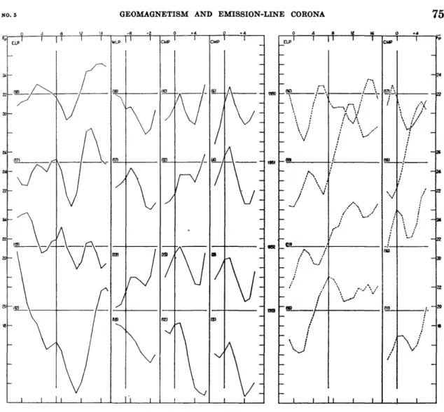
The green line, \5S08, [Fexiv].—We determined mean Kp values for days —4 through + 16 around zero days defined by the ELP of the 10 percent, 20-10 percent, and 30-20 percent of the strongest and the weakest 5303 intensities within each of the four time periods.

Since we did not wish to include any given intensity in two different categories, the percent limits are necessarily only approximate.

To obtain an over-all result for the 45 months we combined the separate results of the four periods, thus taking account of the decreasing general level of 5303 activity during these years.

The geomagnetic activity, Kp, increased from 1950 to the spring of 1952 and decreased there- after. We shall examine the 45-month result first, and then compare the results of the individual periods.

Figure la,b shows the average values of Kp for the 45-month period. The sample size for each of these curves is approximately 125. The average value of Kp for the period is 22.65, as indicated on each curve.

In the period studied the standard deviation of a single daily Kpsxxm is 9.87, so that the ordinary standard error of the mean would be

<r=9.87/ViV, where Nis the size of the sample.

To take account of the positive autocorrelation known to exist between the Kp's for lags of 1, 2, 27, and 54 days, however, the ordinary standard error of the mean must be increased by factors involving the autocorrelation coefficients.

The mathematical definition of the variance (stand- ard deviation squared) of a variable x, in terms of "ex- pected values," is

**=E[x-E(x)]*. (3) E(x) is the expected value of x, or the mean TO. We call o*Jthe second moment about the mean. To get the vari- ance of x=ZxilN, we replace x by * in equation (3).

Whence

(4)

When we assume independence between x, and the second term becomes zero and we have

where <rz is the ordinary standard error of the mean.

When Xi is not independent of xit we define

E (xt—TO) (xt—TO) = p j o1

where p j = t h e autocorrelation coefficient of lag \j—i\.

Shapley (1947), working with the autocorrelation of the magnetic character figure C, found correlations of about 0.5 for 1-day lag, 0.2 for 2-day lag, and negligible correlation for a lag of 3 days. He also found strong autocorrelation in the 27-day recurrence tendency, so we consider both the 27-day and the 52- day lag correlations. Accepting his figures as adequately representing the autocorrelations existing in our sample, we have used 0.5 and 0.25 as the correlations for lags of 27 and 54 days respectively. We then listed all values from which we calculated our 10 percent maximum and 10 percent minimum, and determined the frequencies of lag 1, 2, 27, and 54 days in our sample. With this information, we may now proceed to use equation (4).

Let

ptf=the autocorrelation coefficient of lag d, and

nd=the frequency of occurrence in sample of days with lag d.

Then

=E[JJ S(*<-TO) J

(5)

From this equation we obtain a' (maximum 10%) = 1.28 a' (minimum 10%) = 1.25.

These values may be compared with 0.88, the ordinary standard error derived under the as- sumption of independence of the Kp's from one another.

As a guide to the significance of the variations in the curves in figure la,b, where relevant, we have drawn dotted lines at a distance of two standard errors (adjusted for autocorrelation, <r') from the mean of 22.65. Although

(13)

12 16

r r

59

12 16 DAVS

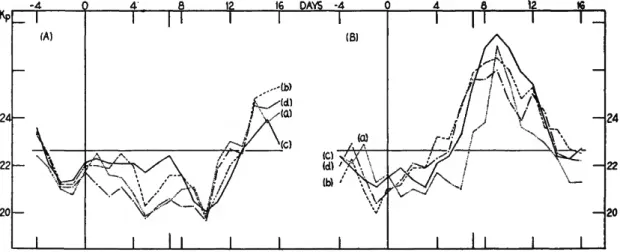
FIGURE 1.—Mean Kp for each day following ELP of various coronal con- ditions, a, Kp after ELP of the 10 percent strongest (a), the 20—

10 percent strong (b), and the 30—20 percent strong (c) intensities of 5303, 1950-53. b, Kp after ELP of the 10 percent weakest (a), the 20—10 percent weak (b), and the 30—20 percent weak (c) inten- sities of 5305,1950-53.

c, 10 percent brightest 5303 intensities for the individual years (3-day running means), d, 10 percent faintest inten- sities for the individual years (3-day running means). Number of cases shown in paren- theses.

(14)

60 SMITHSONIAN CONTRIBUTIONS TO ASTROPHYSICS

this criterion of significance is not exact when applied to the results obtained by the superposed epoch method of analysis, it should provide a fairly reliable guide for judging the results.

Figure la shows that strong 5303 corona on the east limb is followed on da}-s 8-12 by a Kp below the mean, although only Kp(-\-lQ) falls outside the 2-standard-error band. This minimum in Kp after CMP of strong 5303 corona agrees with the result of Kiepenheuer (1947) and appears also in the curves of Shapley and Roberts (1946) for the previous cycle. On the other hand, we find no indication of the maximum around day E L P + 4 that showed so prominently in the curves obtained by Shapley and Roberts in the previous cycle. The patterns of Kp'a after ELP of strong, very strong, and moderately strong 5303 intensities do not differ significantly from one another.

Even the 5 percent strongest intensities failed to produce any significant rise in Kp around days + 7 to 8, such as that found by Wald- meier (1939, 1942) and by Kiepenheuer (1947) for "very strong" corona.

From line (a) of figure 16 we see that weak 5303 corona on the east limb of the sun is followed on days 7-12 by Kp significantly above the mean, with a maximum on day + 9 . Kp (+9) is very close to four standard errors (<rf) above the mean, while Kp (+8) and (+10) are almost three standard errors above the mean, so that this result appears highly significant.

The most probable time for a geomagnetic disturbance, in this phase of the solar cycle, is two days after CMP of a weak coronal region, a conclusion in general agreement with the results of Smyth (1952) and of Bruzek (1952). The 5 percent weakest 5303 intensities give a curve very similar to the 10 percent curve shown.

The effect, however, rapidly disappears with increasing 5303 intensity, being very slight for the weak 20-10 percent group and disappearing entirely for the weak 30-20 percent group of intensities. Thus the moderately weak corona shows no relation to Kp (line (c) of figure 16);

while the moderately strong corona shows a relation similar to that of the strong corona.

Comparison of results from two or more independent samples of data provides an im- portant test for the reality of the results of any

superposed epoch analysis. With this in mind we examined the results of the four time periods (see p. 57) separately. Because of the smaller samples, these curves are less smooth than the 45-month curves. In order to emphasize the principal trends and minimize the irrelevant minor fluctuations we_plottcd these results as 3-day running means, Kp. Figure lc shows the values of Kp following ELP of strong (10 percent) 5303 coronal regions for the four periods, and figure Id shows the values of Kp following ELP of weak (10 percent) 5303 coronal regions. Mean Kp's are shown for each period.

Looking at figure lc we see that the curves of Kp following ELP of strong 5303 intensity- differ considerably from year to year. The Kp's for the first and fourth periods are con- spicuously below the means for these periods.

The second period curve rises more or less continuously after ELP of the strong corona.

The curve for the third period resembles rather closely the results found by Shapley and Roberts in the preceding cycle, and shows a strong maximum in Kp on day 3. Period three covers the time for which Trotter and Roberts (1952) and Muller (1953) noted a return of the eastern-hemisphere effect. Be- cause this effect does not appear in our other three periods—and for reasons to be seen in Part II—we are inclined to doubt the existence of any physical connection between the 5303 corona on the eastern hemisphere of the sun and the M-region responsible for the rise in Kp.

One feature common to all four curves in figure lc is a tendency for a dip in the Kp values 9-12 days after ELP of the bright coronal regions.

While the tendency is present in each curve, in some cases it is very slight and not particularly convincing.

In figure Id the curves of Kp following ELP of weak 5303 intensity are very similar in shape for all four periods, particularly after day 5.

A conspicuous maximum occurs in each period 9-11 days after ELP of the faint corona.

The relationship between 5303 intensity and geomagnetism can be approached, alternatively, through a study of the frequency distributions of Kp following ELP of various coronal conditions. This approach, as Shapley and Roberts (1946) have pointed out, serves to reduce the possibility that one or two very intense

(15)

storms might dominate the shape of the curve, particularly when the sample size is small.

We were particularly interested, of course, in the extremes of 5303 and in the high values of Kp. Because of the tendency to weak Kp on day 10 after ELP of strong corona, the distribution of weak values of Kp is also of interest. We determined, for each time period, the fraction of strong corona on the east limb that is followed by (a) Kp> 30 and by (b) Kp< 12, and the fraction of weak 5303 corona that is followed by (c) K » 3 0 and by (d) Kp<\2. For comparison we computed the fraction of strong and of weak intensities of 5303 which should be followed by strong or weak Kp, if there were no connection between 5303 intensity and Kp. This "expected fraction" is essentially the number of days with Kp~>30 (or of days with Kp< 12) in the period divided by the total number of days in the period.

The results agree well with those found by the previous method. Result (a) is quite similar to figure lc.

The four periods do not agree with one another, except that the observed fraction tends to lie below the expected value (or in period 3 to decline toward it) after CMP of strong corona. Group (b) shows, in each of the four periods, a fairly clear tendency for the observed fraction of weak Kp to rise above the expected value 0-4 days after CMP of strong corona. Result (c) is substantially in agreement with figure Id. The observed fraction lies significantly above the expected fraction 1-4 days after CMP of weak corona in each of the four periods; that is, strong Kp follows CMP of weak corona significantly more frequently than would be expected in the absence of any actual relation between these phenomena. Category (d) shows a systematic tendency in each period for the observed fraction of weak Kp to fall below the expected value 0-5 days after CMP of weak corona.

To investigate the effect of the threshold cor- rections and the interpolations on our results, we calculated mean Kp'a for the 10 percent maximum and minimum 5303, using three different sets of data: (a) the Sac Peak observed intensities, uncorrected for plate thresh- hold, (b) the Sac Peak observed intensities, corrected to plate threshold five, and (c) Sac Peak corrected intensities plus intensities derived from Climax observations and interpolated intensities. Figure 2 shows the results for the 10 percent maximum and 10 percent minimum 5303 intensities. For comparison, the graph includes similar calculations made for the quantity used by Shapley and Roberts (1946), namely the (d) single maximum intensity of 5303 observed at Sac Peak and corrected to plate threshold five.

While the four curves differ in detail and in smoothness, each indicates the same general results, a minimum in Kp 10 days after ELP of strong 5303 and a maximum in Kp 9 days after ELP of weak 5303 regions. We found no statistically significant differences between the four curves for either the strong or the weak 5303 cases.

After ELP of strong 5303 intensities, curves (a), (b), and (d) show a secondary minimum on day 5, followed by a slight rise in Kp around days 7-8. This rise may be a trace of the effect observed by Waldmeier (1939,1942). We recall

Kp

24

22

20

-4 C _ 1

(A)

—

— 1

)

\

\ 4

1

"~"\ \ /

|

8 121 1

\ 1 •/

i i

p 7

16

1

.-(b) /(d) /(ai

DAVS

(O (d) (b) -4

1

(B)

(a)

m

A A

1

c

J

•

4

1 |

I h

v /

8

1 W o / \

1

12

1 \

i

16

1 _

—

V ~

\ •

\

—

1 - 2 4

— 22

— 20

FIGURE 2.—Mean Kp following ELP of strong (A) and weak (B) 5303 intensities. The curves show the results from coronal intensities uncorrected for threshold (a), corrected to plate threshold five (b), corrected and interpolated (c), and the tingle maximum observed intensity (d).

(16)

62 SMITHSONIAN CONTMBUTIONS TO ASTROPHYSICS

that Denisse (1952, 1953) found evidence, from radio-noise observations, for two types of solar active centers, those (R) that produce geomagnetic storms and those (Q) that reduce corpuscular radiation. The curves of Kp following ELP of strong corona are therefore probably a composite of these two types of active centers. From the behavior of the composite, we infer that o-type centers were probably more numerous than R-type centers during the interval covered by our study. Note that this rise of Kp around CMP is present also in figure la and more or less in the four curves of figure lc.

Correlation coefficient.—To compute the coefficient of correlation between Kp and coronal intensity we divided the data into our usual four time periods. For each period we sorted the cards by 5303 intensity into ten equal groups, and assigned intensities on a new arbi- trary scale of 1 to 10. This change in the 5303 scale was made in order to remove the effect of the progressive decline in coronal intensity over the 45 months. In the usual way we then computed the correlation between the 5303 intensities on the 1-10 scale and Kp (—2) through Kp (+15). Figure 3 shows the correlogram of the average correlation coefficients for the four periods. The correlations are very close to zero except on days 7-13 when they become negative. The largest correlation, —0.18, occurs for Kp (10), indicating once again a

•10

DAYS

time lag of about 3 days between CMP of a strong or weak coronal region and its maximum geomagnetic effects.

The red line, X6374, [Fe x].—We determined mean values of Kp for days —4 through +16, as shown in figure 4, around zero days defined by ELP of the strongest 10 percent and of the weakest 10 percent of the 6374 values; the data from Sacramento Peak and those from Climax were used separately. As with the green line, the percent limits with the red line are necessarily only approximate. To obtain the over-all result shown in the figure for the 45 months, the separate results of the four periods were combined.

Figure 4 indicates, with a general similarity between the Climax and Sac Peak curves, that ELP of strong (10 percent) 6374 corona tends to be followed on days 8-9 by a Kp significantly below the mean. Examination of the years separately supports this conclusion. On the other hand, following ELP of weak 6374 the Kp curves are very irregular and lack any significant features; the strong rise in Kp following CMP of weak 5303 intensities is entirely absent for 6374. Outside of active

- 4

FIGURE 3.—Coefficients of correlation between 5303 intensity and Kp, with lags in Kp of —2 to + IS days after coronal ELP.

20

FIGURE 4.—Mean Kp following ELP of strong (a) and weak (b) 6374 intensities, from Sacramento Peak (SP) and Climax (Cx) data.

(17)

regions the intensity of the 6374 line appears to be more uniformly distributed than that of 5303. Therefore minima are perhaps less precisely defined for 6374 and no relation with Kp should be expected.

In general we conclude that Kp shows a substantially closer relation to the intensity of the 5303 line than to the intensity of the 6374 line.

Green line and red line, simultaneously.—

In investigating the effects of the two lines simultaneously, we used only Sacramento Peak red line intensities and the green line intensities corrected to standard threshold.

We determined mean values of Kp for days

—4 through +16 around zero days defined by

22

20 -

various combinations of the two lines, with the results shown in figure 5a, b.

The top curve of figure 5a shows that when both coronal lines are strong, Kp declines quite smoothly (heavy line) from day 3 to a minimum on day 10 which is deeper than any of the minima obtained by using only one coronal line. Days 8-10 have Kp two or more standard errors (cr') below the mean value of 22.65. The asymmetry of the curve about its minimum probably reflects the tendency of Kp to rise more rapidly than it declines. To facilitate comparison we include the mean Kp following ELP of strong 5303 corona and of strong 6374 corona, each computed as before without regard to the behavior of the other line. We suggest also comparison with figures la, 2, and 4. Most noteworthy is the disappearance of the small rise in Kp around days 6-8 when both lines are used; this rise we attribute to storm-producing active centers as distinguished from the more common

22 -

20 -

a

FIGURE 5.—Mean Kp following ELP of various combinations of red and green line intensities, a, Kp after ELP of regions with- the two lines in agreement: line (a), strong 5303 intensities (20 percent) and strong 6374 intensities (30 percent), 108 cases?

line (b), weak 5303 intensities (20 percent) and weak 6374 intensities (30 percent), 83 cases; results for each line alone included for comparison, b, Kp after ELP of regions having one line strong, the other not strong: curve (c), strong 5303 (20 percent) and weak 6374 (30 percent) intensities, 11 cases; curve (d), strong 6374 (30 percent) and weak 5303 (20 percent) intensities,.

23 cases; curve (e), strong 5303 (20 percent) and not-strong 6374 (lower 70 percent) intensities, 66 cases; curve (0, strong 6374 (30 percent) and not-strong 5303 (lower 80 percent) intensities, 111 cases. (Curve (a) is reproduced from figure 5a for comparison.)

(18)

64 SMITHSONIAN CONTRIBUTIONS TO ASTROPHYSICS VOL. *

(in this period) storm-inhibiting active centers. ThuB the curves of figure 5a may have special interest.

The top curves of figure 56 show the mean Kp'a following ELP of coronal centers in which one line is strong and the other weak. The curve when both lines are strong is included for comparison. The results are surprising. When the green line is strong and the red line weak, Kp is above the mean on days 3-11;

when the red line is strong and the green line weak, Kp is above the mean on days 2-10; whereas when both lines are strong Kp is below the mean on days 4-12. While these differences appear to be statistically significant, we should keep in mind that the sample sizes are small. The bottom curves of figure 5b show the mean Kp'a following ELP of coronal centers in which one line is strong and the other line is not strong.

While neither curve (e) nor (f) deviates significantly from the mean Kp, each appears to differ significantly from the case of both lines strong.

The bottom curve of figure 5o shows that no im- provement over green line alone is obtained for the case of both lines weak. This result is perhaps to be expected since the weak red line alone shows no re- lation to Kp.

The interpretation of the results shown in figure 5a, and b, is not at present clear. How- ever, the curves do indicate that the red as well as the green line should be considered in future studies of the relations between geomagnetism and coronal intensity, and that some improvement in predicting the geomagnetic effects of an active center might result from attention to the relative intensities of the two lines.

The yellow line, X5694.—The rare appearance of the yellow line in the coronal spectrum appears to indicate a center of unusual activity.

Waldmeier (1945), Roberts (1952), and Dolder (1952) have pointed out the frequent association between 5694 emission and small, highly active and sharply curved prominences of the sunspot type. They find evidence also for a close association between 5694 emission and solar flares (especially Dolder, 1952).

A search of the CRPL Bulletins revealed that the yellow line was observed at Sacra- mento Peak and/or Climax on 22 occasions between February 1950 and December 1952, 12 times on the east limb and 10 times on the west limb. We omitted three cases occurring in relatively high latitudes in 1953. Figure 6 shows the mean Kp's associated with regions of yellow line emission. The mean Kp for

the period covered by the 22 appearances of the yellow line is 22.65. Because of the small samples the curves are very irregular and the standard errors are large. Most of the fluctuations are not common to the east and the west limb curves and therefore should not be considered significant. However, each curve does show a maximum in Kp around CMP

FIGURE 6.—Mean Kp following ELP of regions of yellow-line emission. The solid curve shows combined results for east and west limb observations; the broken curves show the results for east and west limb appearances separately.

of the region emitting the 5694 radiation. The individual maxima occur on days ELP + 8 and WLP —5, while the maximum of the composite curve occurs on day 7. This maximum does not attain two standard errors from the mean.

To investigate further the relation between Kp and 5694, we determined the frequencies of Kp > 3 0 , 20-30, and < 2 0 on days —2 through + 4 around CMP of yellow-line regions, shown in table 1.

(19)

65

TABLE 1.—Frequencies of Kp around CMP of yellow- line regions

Kp\CMP - 2 - 1 0 +1 +2 +3 +4

Kp>30 20>Kp>20 Kp<20

3 8 11

3 9 10

10 5 7

10 8 4

6 11 5

7 5 10

6 7 9

%Kp>30 14 14 45 45 27 32 27

A chi-square test indicates that the deviations of these frequencies from the expected values are not quite statistically significant; that is, they provide insufficient evidence to reject a hypothesis of independence between Kp and 5694. The last row of table 1 shows the percent of 2Cp>30; the individual values may be compared with a mean frequency of 24 percent for the three years in which the yellow line emissions occur.

While none of the yellow-line results can be declared statistically significant, the above tests do not take account of the location of the deviations from the mean or expected values, i. e., of the fact that the rise in frequency of strong Kp occurs when the yellow line region is on the central meridian. Moreover, yellow line emission appears to be relatively short- lived. Only two of the regions in our sample showed 5694 on both ELP and WLP; (in seven cases coronal observations were obtained on only one limb). Therefore, probably not all of the regions were emitting 5694 radiation when they crossed the central meridian. Certainly the changes in the frequency distribution of strong Kp are in the direction and the position to be expected if yellow line regions tend to produce geomagnetic storms. The results are also in general accord with recent findings by Denisse and Simon (1954) for yellow line regions in the period 1946-52. From the present small sample, however, we can draw no definite conclusions.

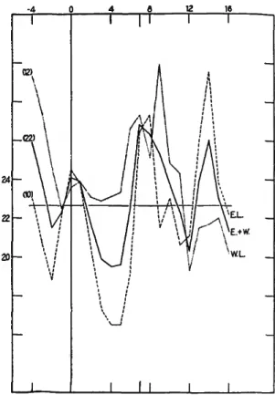
Green line intensity around zero-days defined by large Kp.—In order to obtain a picture of the average distribution of 5303 intensity as a function of longitude on the face of the sun at the time of geomagnetic storms, we prepared an inverse deck of IBM cards containing east limb intensities for days CMP —7 through + 9 (ELP —14 through +2), and west limb intensities for CMP —9 through + 7 (WLP —2 through +14). Using these cards we first calculated the average intensity of 5303 around zero days defined by the maximum 20 percent of the Kp's. Examination of the results for

the 45 months revealed that the 5303 intensity tended to have a minimum on the central meridian of the sun 2-4 days before the occurrence of geomagnetic storms. This minimum appeared in each of the four time periods.

To determine whether sporadic and recurrent geomagnetic storms appeared to be associated with different patterns of coronal intensity we selected, from the lists published regularly in the Journal of Geophysical Re- search, those storms observed to have a sudden commencement (sc) at ten or more observatories. We omitted six storms that appeared clearly to be members of prominent M- sequences. For the remaining 38 storms we computed the pattern of 5303 intensity, shown by line (a) in figure 7. The average intensity was determined from six-month averages weighted by the number of sc-storms occurring in that six-month period. As figure 7 shows, nonrecurrent sc-storms apparently tend to be associated with above-average intensity of 5303 emission around the central meridian of the sun, but no clear time lag can be determined from our graph. The width of the maximum may perhaps arise from the tendency of sporadic storms to be associated with flares; the flares presumably occur in C-regions which need not be at the central meridian of the sun.

We also selected nine of the more prominent recurrence sequences, which gave 58 M-storm epochs, with the zero day defined by the onset

+8

16 —

FIGURE 7.—Mean pattern of S3O3 intensity at various posi- tions on the solar disk: at times of sporadic sc-storms, line (a); of M-sequence storms, line (b).

(20)

66 SMITHSONIAN CONTRIBUTIONS TO ASTROPHYSICS

of the storm. Figure 7, line (b), shows the resulting average distribution of 5303 intensity on the sun. M-type storms tend to be preceded by a minimum in 5303 intensity on the central meridian of the sun 1-2 days before the onset of the storm. The intensity of 5303 crossing the central meridian is below average from 3 days before to 5 days after the onset of the storm. Since each storm is represented only once, the time lag here should be rather precisely defined. The intensity is above its mean 4-9 days before the onset of the storms and drops quite sharply, a drop that corresponds to the relatively sharp if not "sudden" onset of the storm. Indeed the shape of the curve, inverted, resembles an M-storm profile.

We conclude that in the period covered by this investigation, nonrecurrent sc-storms tend to be associated with bright or at least moderately bright 5303 emission and not with weak 5303 areas. However, more C-regions appear to inhibit storms than to produce them. On the other hand, M-regions seem to be associated with regions of weak 5303 corona, with a lag of 1-2 days between CMP of the weak coronal region and the onset of the storm.

Hdiographic latitude of the earth.—In the introduction, we mentioned the well-known tendency of aurorae and geomagnetic storms, especially the recurrent storms, to be most intense around March and September. No satisfactory explanation of these seasonal effects has been given, but most attempts associate the maxima in geomagnetic disturbance either with the equinoxes (i. e., with the geographic latitude of the sun), or with the heliographic latitude of the earth. Following the termi- nology of Bartels (1932) we may call these ex- planations equinoctial and axial, respectively.

In this paper we consider primarily the axial hypothesis, since it is the more susceptible to investigation with our data and, we believe, is the more plausible.

Because the plane of the earth's orbit is inclined 7.2° to the solar equator, the heliographic latitude of the earth varies from 7.2° north of the solar equator about September 7, to 7.2°

south of the solar equator about March 5.

Thus we see a maximum area of the sun's northern hemisphere in September and a maximum area of the southern hemisphere in March,

at approximately the times of greatest geomagnetic activity. The geomagnetic activity tends to be at a minimum around the times when the earth is crossing the heliographic equator.

Apparently solar corpuscles intercept the earth more readily when the earth is farthest removed from the equatorial plane of the sun. On the other hand, the geomagnetic maxima and minima appear to lag behind and to fall closer to the equinoxes and solstices than to the axial parameters (Bartels, 1932).

The usual axial explanation is based on the fact that spots occur most frequently in heliographic latitudes 10-15° while the equatorial belt contains few spots. If the corpuscular streams start from the spot belts and leave the solar surface in a radial direction, corpuscles from the northern and southern belts are most likely to intercept the earth in September and March respectively. However, as we shall discuss later, a relation with the latitude of maximum spottedness is not the only possibility for an axial explanation.

The March and September maxima in geomagnetic activity have not been adequately investigated. Bartels (1932) studied the relation between facular area in the northern and southern hemispheres and geomagnetism. His results offered no support to an axial interpretation. Since he used only monthly means of facular areas and of the geomagnetic index, however, his results are not necessarily significant. The effect of the heliographic latitude of the earth in relation to active centers on the sun has not, so far as we are aware, been studied on a daily basis. We made an explor- atory study of the problem from two directions.

Active centers or C-regions.—We had recorded, on the original IBM cards, the latitude of the brightest single 5303 intensity for the day.

The value of this latitude we took to indicate whether the associated C-region was located in the northern or in the southern solar hemisphere. When two C-regions occurred simultaneously, one on either side of the equator, we disregarded the region with the weaker maximum; days with maxima of equal intensity in north and south were omitted.

We designated as "favorable" (f) those C- regions on the same side of the solar equator as the earth, and as "unfavorable" (u) those