Introduction
Motivation
Mitigation of methane emissions has emerged as a crucial approach to combating anthropogenic climate change in the coming decades. Accurately attributing the sources of methane emissions and the drivers influencing atmospheric methane trends is therefore crucial for the effective implementation of climate change mitigation strategies.
Methane Sources and Sinks
As a major contributor to radiative forcing, methane, which accounts for a third of radiative forcing, harbors a global warming potential 85 times more potent than carbon dioxide over 20 years (W. Collins et al., 2022; Shindell, Fuglestvedt, and W.J. Collins , 2017). As a result, limiting methane emissions not only helps limit climate change, but also improves air quality (Fiore et al., 2008).
Proxying Methane Processes
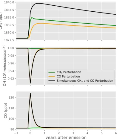
Because MCF has no other destruction pathways in the troposphere, changes in loss frequency can be attributed to changes in OH concentrations (Montzka et al., 2011; Patra, Krol, et al., 2021). 13CH4 has played an important role in understanding methane trends (McNorton et al., 2016; Alexander J. Turner, Christian Frankenberg, Wennberg, et al., 2017).
The Methane Stabilization Mystery
This shift toward lighter methane indicates either an increase in emissions from biogenic sources of methane, such as agricultural or microbial activities (Schaefer et al., 2016; Nisbet et al., 2016), or a decrease in emissions from isotopically heavier sources, such as biomass burning. (Worden et al., 2017). However, these figures assume that the isotopic signature of certain sources remains spatially consistent and constant over time, which may not always be the case.
Sensing Methane
A comprehensive global observing system, capable of monitoring both natural and anthropogenic emissions, along with an improved understanding and precise measurements of OH sinks, is needed to fully characterize methane emissions and trends. In particular, the tropical atmosphere is where most uncertainty in methane emissions resides, in addition to where most methane destruction occurs, given the abundance of the OH radical.
Methane Spectroscopy and Retrievals
Errors in the modeling of these line shapes will lead to errors in the retrieval of greenhouse gas concentrations. In Chapter 4, I delve into the impact of environmental influences on the accuracy of methane and CO2 extraction.
Thesis Outline
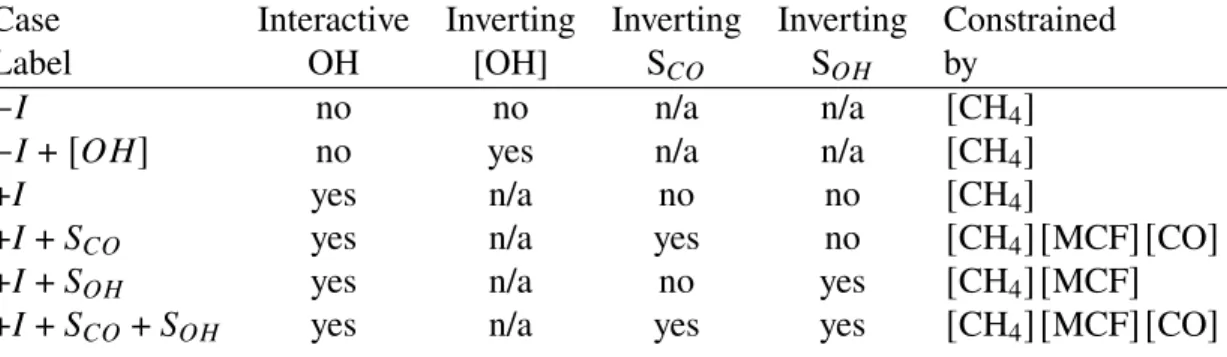
In the non-interactive case (-I) the OH concentrations are fixed, so methane emission inversions only respond to changes in methane concentrations, while in the interactive case (+I) methane emissions adapt to changes in methane and OH concentrations. Gradients of average CO2 concentrations in the atmosphere at the regional scale are about 2% (8 ppm) (Thompson et al., 2012).
Effects of Coupled Chemistry on Methane Emissions
Abstract
Using a coupled chemical box model, we show that neglecting these effects can lead to a 50% bias in calculating methane source perturbations over several decades. Finally, we quantify the inclusion (or exclusion) biases of related chemistry in the context of recent methane and CO trends.
Background
However, the combined chemistry of carbon monoxide (CO), methane, and hydroxyl radical (OH) can modulate methane lifetime, which is often ignored in methane flux inversions; and the impacts of neglecting these feedbacks have not been quantified. Given these uncertainties, in addition to the contradictory hypotheses discussed here, the question remains: "how do simplifying assumptions on the associated chemistry affect estimates of methane emissions?".
Hemispherically Averaged Concentrations
2.1, each 𝑋𝑖 represents the concentration of species 𝑖 (e.g. methane, CO, OH, NO𝑥) that could affect methane lifetime. Here we focus on the coupled chemistry of methane, CO, and OH using a two-hemisphere box model with coupled methane, CO, and OH chemistry (Prather, 1994; Prather, 1996).
Constructing the Forward Model
Chemical Feedbacks Result in Extended Methane Lifetime
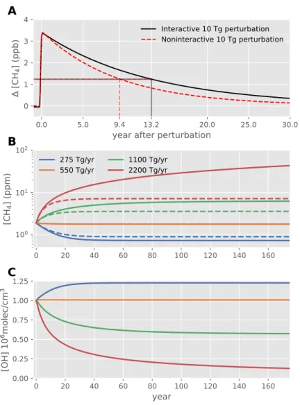
As our mandated emissions become larger, the difference between the steady-state methane concentrations in the interactive and non-interactive cases becomes even more distinct. In the case of 2200 Tg/yr, the lifetime and steady-state lifetime differ by more than a factor of three, which is due to the reduction of OH (Figure 2.1c).
Effects of El Niño on Methane Concentrations
For emissions greater than the contemporary case of 550 Tg/yr (Saunois et al., 2016), the interactive chemistry cases have much higher steady-state methane concentrations than their non-interactive counterparts, because methane concentrations affect OH. Methane concentrations (panel B) and OH concentrations (panel C) are shown for our steady-state test, where emissions are fixed at and 2200 Tg/yr for both interactive (solid lines) and noninteractive (dashed lines) chemistry.
Inverting for methane Emissions
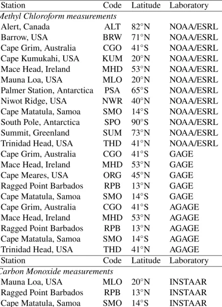
Kabo Grim, Australia CGO 41◦S NOAA/ESRL Kabo Kumukahi, VS 20◦N NOAA/ESRL Ulo ti Mace, Irlanda MHD 53◦N NOAA/ESRL. Ragged Point Barbados RPB 13◦N GAGE Kabo Matatula, Samoa SMO 14◦S GAGE Kabo Grim, Australia CGO 41◦S AGAGE.

Timescale for INcluding INteractive OH Chemistry
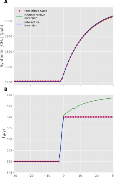
Ragged Point Barbados RPB 13◦N INSTAAR Cape Matatula, Samoa SMO 14◦S INSTAAR .. mance of our inversion, and 2) to calculate the error associated with neglecting interactive OH chemistry in an inversion as alluded to in ( Prather and Christopher D. Holmes, 2017). However, inverted methane emissions, in our non-interactive inversion, are consistently higher after our prescribed emissions increase (Fig. 2.3b), reaching an overestimate of about 5 Tg/yr after only 10 years after the emissions change, which is 25% of the perturbation .
Emissions Estimates with Observed Concentrations
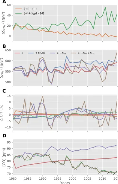
When we assume a variable OH source (+I+𝑆𝑂 𝐻), variability in methane emissions is attenuated because OH production and recycling can compensate for variability in OH concentrations. Also, the fit for CO emissions (+I +𝑆𝑂 𝐻 + 𝑆𝐶 𝑂) further mitigates the variability of methane emissions because CO emissions are also allowed to compensate for the variability of methane emissions.
Summary and Recommendations
For example, a +2% increase in lower stratosphere.. water vapor corresponds to a -2% decrease in the stratosphere-troposphere exchange time. In the previous section, we found that retrieval errors correlate strongly with water vapor concentrations.
Stratospheric and ENSO Impacts on Tropospheric Methane Emis-
Background and Motivation
Water vapor in the lower stratosphere comes from upwelling from the troposphere and photochemical oxidation of methane in the stratosphere. H2O concentrations in the lower stratosphere are linked to the variability of stratosphere-troposphere exchange (Fu et al., 2015; Lu et al., 2020; Randel and Jensen, 2013).
ENSO and Its Impact on Methane Emissions
Although increased lower stratospheric water vapor concentrations would intuitively indicate stronger tropical upwelling and stratospheric circulation, most of the effects of stratospheric-tropospheric exchange actually reduce H2O concentrations in the lower stratosphere due to increased upwelling of dry air entering the lower stratosphere (Fu et al., 2015; Lu et al., 2020). The Brewer-Dobson Circulation is primarily responsible for this transport, with the ascending branch driving the transport from the troposphere to the stratosphere in the tropics and the descending branch responsible for the transport from the stratosphere to the troposphere in the high latitudes.
Observational Constraints
Tracer Growth-rate Correlations
Therefore, N2O has been proposed as a proxy to distinguish between tropospheric and stratospheric air, and the N2O growth rate has been shown to be modulated by inter-annual variations in the strat-trop.

Lower Stratospheric Water Vapor Observations Proxy Stratosphere-
This implies a continuously increased stratosphere–troposphere exchange during this period, which likely contributed to the observed reduction in methane emissions and OH variability. In the following years, there was a slight further decrease in water vapor concentration by -2.1%, indicating a continuous increase in the exchange between the stratosphere and the troposphere.
Chemical Box Model
This increase suggests a dramatic decrease in stratosphere-troposphere exchange, in line with the observed increase in methane emissions, indicating that the stratospheric sink of methane decreased, leading to even more methane growth. water vapor corresponds to a -2% decrease in the exchange time between stratosphere and troposphere. This allows us to quantify the effect of variations in stratosphere-troposphere exchange time on methane emission inversions and OH concentrations.
Results and Discussion
El Niño years were associated with significant changes in methane emissions, OH variability, and lower stratospheric water vapor concentrations. El Niño also appears to accelerate stratosphere-troposphere exchange, as indicated by lower stratospheric water vapor concentrations.
Conclusions and Recommendations
During several weeks of using DCS in the field, we found deviations of up to 2% in methane concentrations and 0.5% in CO2 concentrations when using different spectroscopic databases. Fourier transform infrared spectroscopy measurements of H2O-broadened half-widths of CO2 at 4.3 m. This article is part of a special issue on Spectroscopy at the University of New Brunswick honoring Colan Linton and Ron Lees.” In: Canadian Journal of Physics87.5.
Towards Laboratory-level Accuracy in the Field: Environmental
Abstract
However, the synthetic retrievals revealed a variable error of 8% in the methane concentration obtained across different lists, mainly due to errors in the pressure expansion. Compared to other line lists, there was a 0.8% variable error in obtaining CO2 concentration, mainly attributable to errors in pressure expansion.
Background
To do this, in Section 4.5 we use DCS to estimate the precision and systematic biases of several spectroscopic line lists. In Section 4.6, we then quantify the impact of environmental variable biases with respect to pressure and temperature errors on GHG retrievals with idealized synthetic retrievals.
Dual-Comb Spectroscopy Technique
DCS has a full-width instrument lineshape at half-max of 4×10⁻⁴cm−1, making the instrument lineshape negligible. The instrument was mounted on a radio tower 30 m above ground along the DCS beam path.
Retrieval Approach
The dry air column density (𝑑𝑟 𝑦𝑐 𝑑) is calculated by multiplying the dry air number density (𝜌𝑑𝑟 𝑦) by the round trip distance (Δ𝑥). Pressure and temperature errors will affect the amount of dry air column and propagate to the derived greenhouse gas concentration.
Greenhouse Gas Spectroscopy
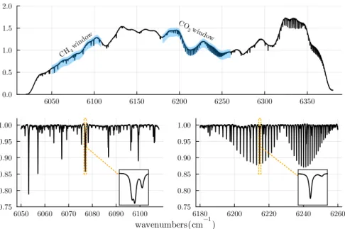
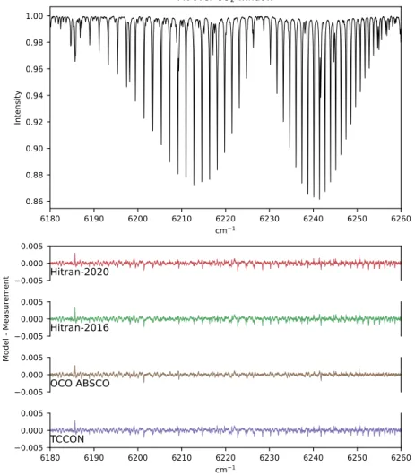
Examining the residuals in panel B, we see that all the tested line lists generally have minimal systematic residuals. The bottom panel shows the residuals with modeled spectra using the Hitran TCCON, 2008, Hitran 2016 and Hitran 2020 line lists.
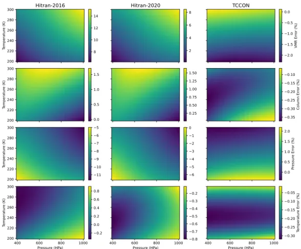
Synthetic Retrieval Experiments
From top to bottom row, errors in concentrations (denoted as VMR), methane column density, reclaim pressure, and reclaim temperature are plotted as a function of pressure and temperature. From top to bottom row, errors in concentrations (denoted as VMR), CO2 column density, reclaim pressure, and reclaim temperature are plotted as a function of pressure and temperature.
DCS Field Retrieval Results
All line lists used here follow very closely with the in-situ reference observations, denoted as black dots. The differences between the different line lists used are small and difficult to distinguish, indicating that the CO2 spectroscopy is in agreement.

H 2 O Broadening
H2O expansion can increase pressure expansion, so we instead calculated an effective pressure (𝑝𝑒 𝑓 𝑓 𝑒 𝑐𝑡𝑖 𝑣 𝑒) to account for additional pressure expansion due to water vapor concentrations. We see that water vapor can have up to 10 pbb (0.05%) impact on methane extraction on days with higher water vapor concentrations.

Summary and Discussion
H2O expansion affects not only CO2 uptakes through the dry air column, but also the density of the CO2 column itself. Considering that neglecting H2O expansion already has a significant effect at 1.5% H2O concentrations, this effect can only be larger in tropical atmospheres where concentrations can be up to 5%.
Implications and Recommendations
Pressure broadening in the 2ν3 band of methane and its consequences for atmospheric measurements”. Broadband frequency references in the near infrared: precise double comb spectroscopy of methane and acetylene”.
Main Findings, Summary, and Recommendations
Overview
As the second most important contributor to greenhouse gas-induced warming after carbon dioxide, methane plays a crucial role in accelerating climate change. Through these advances, my dissertation has increased our understanding of methane destruction processes and moved the field of remote sensing of greenhouse gases toward more accurate and reliable measurements.
Main Findings in this Dissertation
I used the accuracy and stability of frequency combs to quantify environmental biases in greenhouse gas spectroscopy. Environmental conditions affect the absorption of GHG radiation, which affects the accuracy of GHG extraction.
Recommendations and Concluding Remarks