We exploit the combinatorial properties of surface maps in free groups to prove several new results on stable commutator length and bounded cohomology. Therefore, in this chapter we present an overview of the stable commutator length, quasimorphisms and surface realizations of free groups.
Stable commutator length
Definition
There is a considerable amount of overlap in the background material required for the various chapters, so it is useful to collect it in one place. If [C] = 0 inH1(G;Z), in which case C ∈ B1(G;Z), the boundary space, then there exists a surface map S → K(G,1) with n boundary components such that images of boundary components in π1(K(G,1)) =Ghart with conjugation classes of thegi.
Extremal surfaces and examples
Quasimorphisms
- Definition
- Duality with scl
- Counting quasimorphisms
- Rotation quasimorphisms
Both the large and small counting quasimorphisms are, as announced, quasimorphisms, and they are homogeneous. Large-count quasimorphisms are easier to compute, but small-count quasimorphisms have a uniformly bounded defect.
Free groups
- Notation
- Stallings graphs
- Subgroups and covers
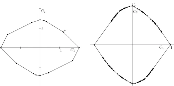
- The scl norm ball
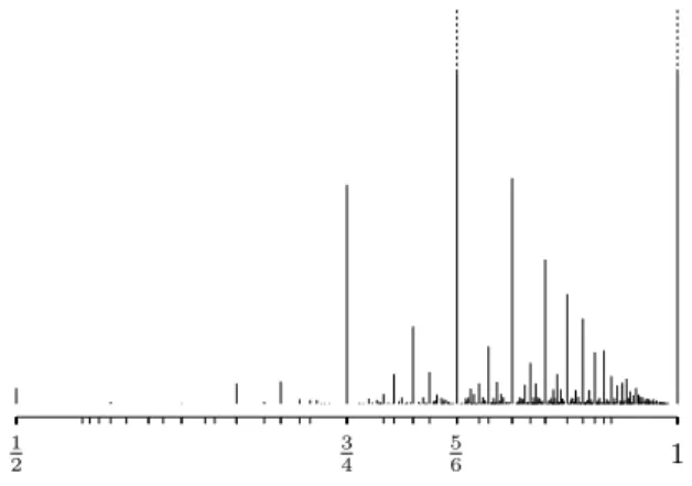
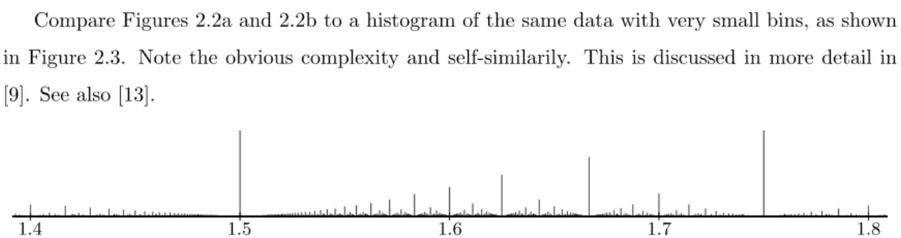
- Pictures of scl in free groups
This is of course also a consequence of the more powerful (and more difficult to prove) fact that finitely generated subgroups of a free group are separable (free groups are LERF) (see [23]). While they are polyhedra, these finite-dimensional slices of the norm ball can be quite complicated.
Fatgraphs
Fatgraphs
Since it is the heart of many of our computational arguments, we record the following corollary of Lemma 2.4.3 as another lemma. In other words, after possible compressions and homotopy, every admissible map is carried by a labeled graph.
Stallings fatgraphs
Surface realizations
- Surface realizations
- Rotation quasimorphisms from realizations
- Cyclic orders and basic surface realizations
- A formula for rotation number
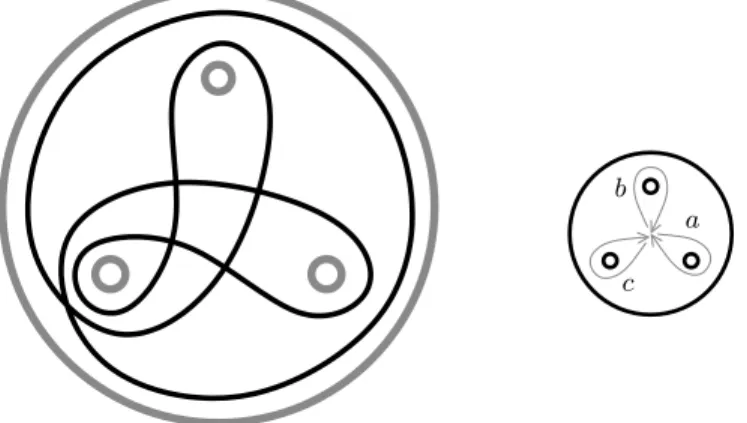
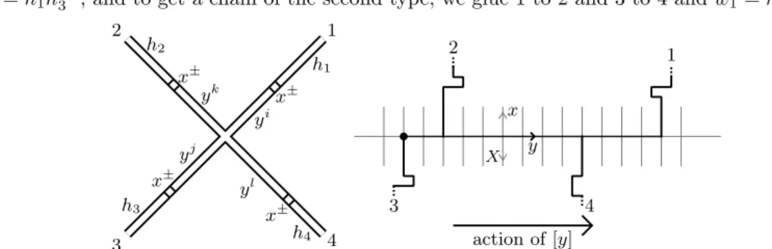
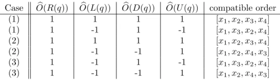
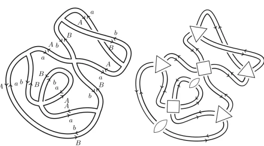
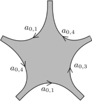
We will denote explicit cyclic orders with square brackets, so [x, y, z, w] gives a cyclic order on the set {x, y, z, w}. If S is a set with cyclic order O, and x, y, z ∈ S, we define the distance between x and y, avoiding that z is the number dz(x, y), so that x and y dz( x, y). )−1 elements in between, if ordered according to the total order Introduction This holds for any non-geometric coverage, so for any finite index subgroup there are infinitely many elements of B1H(H) whose scl strictly decreases under the (injective) inclusion map. Suppose that ϕ:F(B)→F(A) satisfies condition (SA) and let Y be a fat graph with ∂S(Y) in the form of ϕ, i.e. such that ∂S(Y) is a collection of cyclically reduced words of the form ϕ(g). Define a random homomorphism of length ≤n as a homomorphism ϕ : Fk → Fl that sends a (fixed) free generative set for Fk to randomly selected elements of F`(≤n) (with a uniform distribution). If w−1 appears in ∂S(Y), then at least half of it must appear as a subword of one of the edges of Y, so the probability that w−1 appears in ∂S(Y) is certainly less than the probability that Yes. The correction term ensures that the length of the shortest word in the support S is the minimum. To prove the lemma, it suffices to show that the error of the non-homogenized quasimorphism is at most 3. The bold circle indicates the base point, and the arrow indicates the tripod that determines the cyclic sequence. Let the standard generating set of F2 be the cyclic sequence [a, b, A, B], and consider the tuple (bAB, bab, baa). We therefore say that the tuple (bAB, bab, baa) is negatively cyclically ordered in the cyclic order on F2 determined by [a, b, A, B]. There will be a unique tripod in the union of the embeddings, and if the tuple (g1, g2, g3) is ordered cyclically in the same way as the generators labeling the tripod, then the tuple is positively ordered. Condition (1) in Theorem 4.2.2 is a simple combinatorial check, provided we have a graph representing φ−1◦g : S → Xk. In addition, if g:S→Xk is a surface map and (φ, O) a realization of the fatgraph of F, it is possible to check condition (1) of Theorem 4.2.2 "all at once", and not at each vertex Separately. Take a maximal subgraph T of S - the remaining edges of S define a set of generators {gi}ki=1 for π1(S). This means that if g and h are such that the product reduces, then the length of the segment that cancels (on each side of the cyclic multiplication) in φ(g)φ(h) is less than Cφ. But if the cyclic orders are different (as in (B)), then whatever the cyclic order associated with the fatgraph realization, it cannot be compatible with both vertices. The most important thing is (4): since g is blocking for φ, we can apply φ to the fat graphs (A) and (B), and we know that the convolution process cannot cross any of the blocking words g (andg−1), so the barrel graph must be folded identically around each vertex. After dealing with any power of φ, either C or C−1 is contained in T and the lemma follows. There are infinitely many commutatorsCinB1H(F2) such that each one divides the set T of geometric faces into two sets; T0, those containing C, and T0, those containing C−1=−C. Of course, we are most interested in the case where Γ does not bind an immersed surface in any realization of F. In anticipation of non-trivial examples of that, we define a vimersion to be a chain Γ ∈ B1H(F ), together with a finite index subgroup G ⊆ F and a discrete, faithful representationρ:F →PSL(2, R) such that (rotρ)GF is extremal for Γ, or equivalently, that TFG(Γ) bounds an immersed surface in the realization of G corresponding to ρ. Simplifying, if we denote a0, a1, a2, b by a, b, c, d, the "interesting" (unbounded parallel) loop in w02 corresponds to the conjugation class ADABDBCDCd. In this cover, ADADBBCDC rises to two loops as shown in the figure, and after filling the four holes and pushing over the bigon, we get a curve isotopic to "interesting". After filling half of the holes in this cover together with the hole corresponding to a0, one copy can be pushed over the bigon to obtain a curve, the isotopically "interesting" component wn−10 , which, together with the corresponding border parallel loops, bounds the immersed surface according to the induction hypothesis. This picture carries over to higher n: the "interesting" component of wn0 lifts up to two loops in a 2-fold cover of Σ0,n+3 "branches" over the puncture corresponding to a0. Furthermore, the transfer of wn bounds an immersed surface in (gives a vimerization with) Gn → π1(Σ0,n+3)whereGn is the subgroup of index n+ 1 inF2, also as above. However, this is equivalent to checking that the intrinsic cyclic order of an exhaustive set of ends E is compatible with the order O gives E. Therefore, an automorphism of G induces a continuous mapping at the ends of F, and a cyclic order on G induces a cyclic order on the ends of F. In the notation above, (rot(φ,O))GF is extreme for C if and only if the cyclic order determined by (φ,O) at the ends of Gis is compatible with the intrinsic cyclic order at ψi E, for allψ1, . This means that we can determine the cyclic order in the image of a triple using only a triple of finite edge prefixes. This gives a view of the edge triplets of F which, like the edges in G, are invariably ordered under F/G. It will suffice to take 3-dimensional slices of the set of all invariant 4-tuples. Then for any cyclic order O onS0 = {sn, si, sj, sm} there exists a λ that the λ-order on S restricts to O. Note that the cyclic order given by the λ-order is tulu , independent when all indices move by the same amount. The assumption that i−n 6= m−j is necessary: if we have equality, there is no λ-order restricted to one of the orders in the third row. If two of the ends are ±y±∞, the shift action of F/Gn always keeps the other end on the same side, and the limit is ±1. The hypothesis of Theorem 4.7.8 can be weakened somewhat, at the expense of purity of λ orders. In this chapter, the rankings of our free groups are not particularly important, so we suppress the subscript notation Fk in favor of the generic F. RecallB1(F) is the space of limits in group homology F, or more explicitly, the space of formal sums of words that are trivially homologous. The space W` is the natural space in which we work if we want to study the dynamics of endomorphism on a certain length scale. In all these cases, we are interested in the space of positive weights, those weights that have non-negative coefficients for each word. A reduced word inF gives a simple path inT`, and φ works on such paths, although the action is not easy, because we have to sharpen the result of applying φ before it yields a path in T`. The expansion condition essentially guarantees that the mean derivative of φ is bounded (and greater than 1) at some path below. We note that an irreducible automorphism expands on a large enough scale for subwords of its invariant lamination. First note that the limit exists because the expression is (not strictly) decreasingly monotonic and bounded below. Note that the cylinder we climb to join the boundaries of Σ will wrap ktimes around the torus of the map of φ; that is, it passes X× {0}a total of times. To prove the other direction, observe that the Mayer-Vietoris sequence from Lemma 5.2.5 states that every representative of αinH2(Fφ) arises as the adjoint of some boundary of the surface C0−φ(C0) with [C] = [C0]. We can use Lemma 5.2.8 to certify a norm-realizing surface, because if φ gives a well-defined action on W`, then the infimum on the right is a finite-dimensional problem, and can in fact be computed using a variation on the algorithm from Theorem 5.1.5. We let Lφ⊆T be the limit set of φ, which is the set of stands in. Similarly, we define Qφ to be the set of quadpods in the image ofφn for alln. In particular, condition (A) from §3.3.3 on the set of words obtained by applying φ to the generators guarantees that φ is expanded. In all cases, there is a cyclic sequence on Q that causes the required signs on all the tripods. By Theorem 5.3.4 it is sufficient to check that a random endomorphism of length n extends to scale K= 1. Note, however, that expansion to scaleK= 1 follows immediately if the targets of the generators have bounded cancellation. Geometric HNN extensions By taking covers, we can assume that the boundaries of Smap with the same degrees toCand−φ(C), so we can glue it together into a closed surface map ¯g : ¯S→Xφ representing a multiple of the homology classα. Using scallop[15] (made easier by walling [32]), we can find a specific example: a genus 1 surface with boundary bb+AbaBBAbaBB. For example, there is a genus zero face (dotted sphere) with 8 boundaries, which bounds twice the chain. Overview Given Γ ∈B1H(Fk), let VΓ be the vector space overQ spanned by all possible labeled polygon pieces and rectangles for Γ. For each pair of central edges, arbitrarily glue the collection of edges of polygon pieces to those edges. By construction it can be cut into the polygon pieces and rectangles we started with, sokv is a cut vector for (S, f). The scylla algorithm for free groups We will denote bygi(x, y) the group of polygon interface edges between two sides labeled with letters x and y. We will denote this by gt(y, z, i, x), where the interface edge is gi(y, z) at index i in a group polygon based on x. Note that any cyclic fat graph bounding Γ can be cut into central polygon pieces, rectangles, and group teeth. Combining Lemmas 6.4.4 and the same proofs as Lemmas 6.2.3 and 6.2.4, we obtain the following analogous theorems. This reduces the number of polygon parts to consider, and causes the cylinder to generate a smaller (non-rigorous) linear program when >320. 25] Ilya Kapovich and Martin Lustig, Invariant foils for irreversible automorphisms of free groups, preprint; arXiv:1104.1265.![Figure 2.7: The basic fatgraph realization of F 3 = ha, b, ci induced by the cyclic order [a, b, A, B, c, C].](https://thumb-ap.123doks.com/thumbv2/123dok/10401507.0/27.918.301.666.84.264/figure-basic-fatgraph-realization-f-induced-cyclic-order.webp)
Isometries and non-isometries of scl
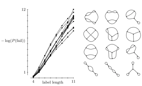
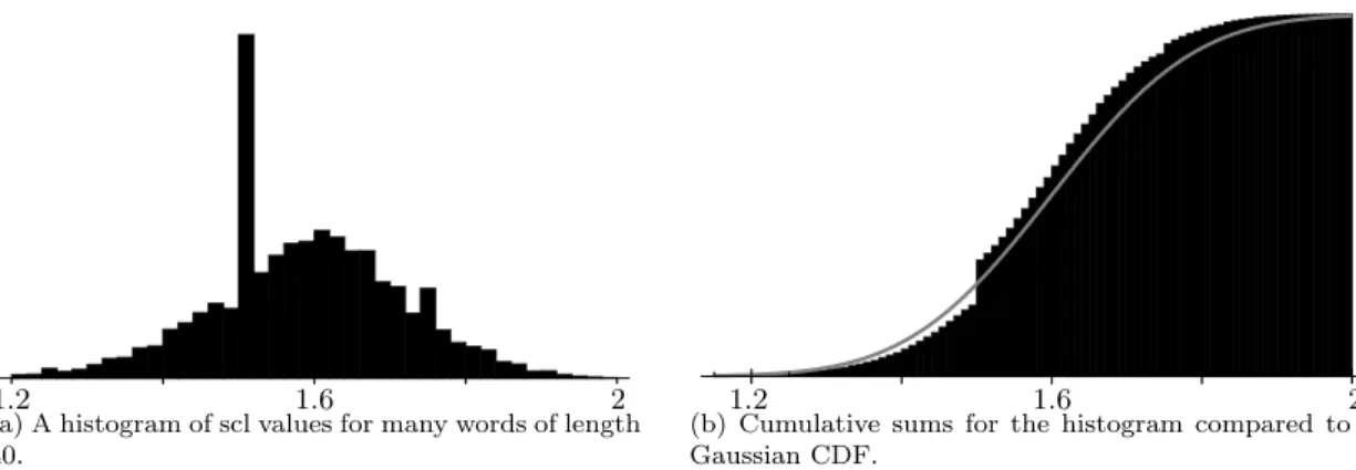
Random homomorphisms are usually isometries
Random fatgraph labelings are usually extremal
Cyclic orders and compatibility
Realizations and immersions
Fatgraph realizations
Surface maps into fatgraph realizations
Examples and consequences
Transfer
Transfer of quasimorphisms
Transfer of rotation quasimorphisms
Example
Symplectic rotation number
Ends
Cyclic orders and the extremality of transfer
Examples
Limit transfers
Limit transfers
Traintracks
Endomorphisms and HNN extensions
Endomorphism actions on traintracks
Norm-realizing surfaces in HNN extensions
Geometric endomorphisms
Tripods and cyclic orders
Geometric endomorphisms
Equivariant rotation quasimorphisms
Norm-realizing surfaces in geometric HNN extensions
Norm-realizing surfaces in geometric HNN extensions
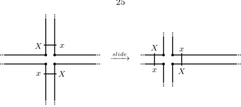
Improving the combinatorial structure in scallop
Generalizing to finite cyclic free factors
The complete scylla algorithm
Complexity and comparison with scallop
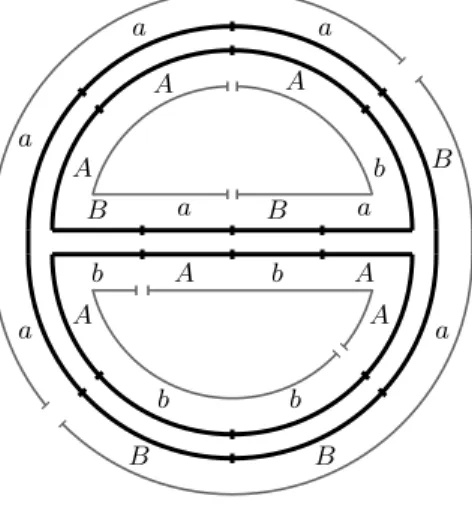
![Figure 2.6: A labeled fatgraph; the induced surface map takes the boundary to the conjugacy class of the commutator [abAB, BaBA] = abABBaBAbb.](https://thumb-ap.123doks.com/thumbv2/123dok/10401507.0/23.918.392.593.77.269/figure-labeled-fatgraph-induced-boundary-conjugacy-commutator-ababbababb.webp)