Three Essays on Information Economics

(1)

Three Essays on Information Economics

Thesis by

Qiaoxi Zhang

In Partial Fulfillment of the Requirements for the degree of

Doctor of Philosophy

CALIFORNIA INSTITUTE OF TECHNOLOGY Pasadena, California

2016

Defended May 4, 2016

(2)

(3)

ACKNOWLEDGEMENTS

(4)

ABSTRACT

The main theme of my thesis is how uncertainty affects behaviors. I explore how agents seek to resolve uncertainty in different environments. In Chapter 1, agents learn from the messages of informed experts in a signaling game. In Chapter 2, an agent learns about a fixed and uncertain physical environment through dynamic experimentation. In the last chapter, agents learn about others’ preferences through the outcome of a central matching mechanism.

Motivated by the question of how opposing political candidates who are policy experts can communicate to voters in a way that helps them win the election, I study a delegation problem with two informed, self-interested agents. Agents make proposals before the decision maker decides to whom to delegate a task. The innovation is that there are multiple issues that the principal and agents care about, and the agents can be vague about any issue in their proposals. Intuition says that agents should be specific about the issues that they are trusted on and vague about other issues. I find the opposite: an agent is disadvantaged by revealing information about certain issues to the decision maker, those on which he is trusted by the principal on. The reason is that doing so enables his opponent to take advantage of this revealed information and undercut him. Essentially, when the principal is on an agent’s side for some issue, that agent does not want to be specific, because it creates a visible target for his opponent to react to. He wants to be vague, because that allows the principal’s ignorance about the optimal action create an insurmountable obstacle for his opponent. As a result, it is to an agent’s advantage to be vague about the issue that he is trusted on.

The second chapter investigates the implication of biased updating in dynamic experimentation such as a firm’s R&D process. People exhibit near miss effect during gambling. For example, if the first two wheels of a slot machine indicate a potential final outcome of jackpot but the last wheel indicates a loss, people are motivated to gamble more. An outcome that is close to a success but is still a failure is called a “near miss.” In this chapter, I explain the near miss effect in a firm’s repeated R&D process. There are two factors that sequentially affect the profitability of R&D, both of which are uncertain. First is whether the R&D team is skilled enough to make a technical breakthrough. If a breakthrough occurs, then a second factor comes into play, which is whether the market demand is high enough to make the product profitable. Moreover, good news for the first stage

(5)

is a prerequisite for learning about the second stage. In each one of the infinite periods, the decision maker of the firm decides whether to involve in risky R&D and observe whether the outcome is a failure (no breakthrough), a success (with breakthrough and high market demand), or a near miss (with breakthrough but low market demand). I assume that the decision maker of the firm learns about the skill of the team properly, but when she updates about the market demand, she updates incorrectly and overweighs her prior. In particular, her posterior about the market demand is a convex combination of her prior and the Bayesian posterior. This bias affects the relative updating of the two factors, which gives rise to the near miss effect: after a near miss is observed, the decision maker values doing R&D more than before although she has received no payoff.

I show that if the decision maker is sufficiently biased and overweighs her prior enough, then she exhibits the near miss effect. I also compare the near miss effect for decision makers with different degrees of biases. As it turns out, the more biased a decision maker is, the more sever she exhibits the near miss effect. However, given the decision maker’s belief about the two factors, the more biased she is, the less she values R&D. Consequently, the value of R&D is highest for a Bayesian.

In the last chapter, I study how well a centralized matching mechanism works when agents do not know others’ preferences. I consider a standard two-sided marriage matching problem, except that agents only know their own preferences. Roth (1989) proved by an example the non-existence of a mechanism with at least one stable equilibria. In his proof, an agent is allowed to report a preference that is realized with ex ante zero probability, which violates the setup of a Bayesian game. Instead, by restricting agents to report only preferences with positive realization probabilities, I show that Roth’s result still holds. More interestingly, as long as agents are allowed to form blocking pairs after a matching outcome is announced, the final outcome is always stable with respect to the true preferences. This means that even when the mechanism fails to produce a stable outcome, it can still release enough information for agents to initialize a blocking pair, which induces a stable outcome.

(6)

LIST OF ILLUSTRATIONS

Number Page

1.1 Only vague about misaligned dimensions . . . 3

(8)

LIST OF TABLES

Number Page

3.1 State of information . . . 82

3.2 ω = a . . . 85

3.3 ω = b . . . 85

3.4 ω = c . . . 85

3.5 ω = d . . . 85

(9)

C h a p t e r 1

VAGUENESS IN MULTIDIMENSIONAL PROPOSALS

1.1 Introduction

This paper studies how competition shapes information revelation. Consider two self-interested agents, Agent 1 and Agent 2, who communicate to a decision maker (DM) about their future actions. Agents have private information about the consequences of actions and can strategically choose to be vague about their actions.

When actions are multidimensional, whether and on which dimension to be vague are the subjects of this paper.

Delegation often involves multidimensional decisions. Consider a parent who chooses between two schools for her child. Many aspects of a school affect a child’s well-being: the physical activity level, the social environment and the cur- riculum, etc. A school can reveal these information about itself, but may not credibly convey whether it is optimal for the child. For example, a school may announce that their students have PE classes twice a week. Without knowing the optimal frequency of PE classes for a child, a parent cannot evaluate how well the school does in terms of physical well-being. In this paper, I show that if both schools know the consequence of PE class frequency, then the school that is stronger in developing students’ physical well-being has an incentive to be vague about their PE class frequency. The reason is, by making a specific announcement of its PE class frequency, it reveals the optimal PE class level to the parent. The weaker school can in turn promise an appropriate PE class level that makes it slightly better overall. In other words, by being specific, a school’s advantage is undermined.

Here is the formal setup. Nature chooses a state of the world. Agent 1 and Agent 2 observe the state, then simultaneously announce proposals. The DM, who does not observe the state, tries to infer the state from the proposals, and selects one agent to implement the decision. The outcome of the decision depends on the state and determines everyone’s welfare. Both the decision and the state are multidimensional.

For each dimension, one agent has an advantage in that his interest is more closely aligned to the DM’s than his opponent’s.

Agents can choose their levels of commitment as well as actions to commit to. They are allowed to be vague about any dimension of their future action by sending a

(10)

null message. Consequently, they have full freedom to take any action if chosen to make the decision. However, they are bound to any specific, non-vague actions that they propose. Since a commitment is binding, it likely reflects an agent’s private information about the state. On the contrary, vagueness gives an agent full freedom to implement his own ideal action without revealing their private information. As a result, commitment and information revelation go together.

I show that vagueness is a natural consequence of competition. Not only is vagueness sustainable in equilibrium, an agent’s vagueness appears on the dimension that he has an advantage on. If he is vague about dimension 1, then the DM believes that he will implement his ideal action without herself knowing what that is. Since she is ignorant about the state, she is free to adopt any belief about it. In particular, she is free to believe that any specific action proposed by Agent 2 is Agent 2’s own ideal action, which is worse than Agent 1’s ideal action. Therefore, the DM’s ignorance precludes any possible compromises by Agent 2 on his disadvantaged dimension.

On the other hand, if Agent 1 is specific about dimension 1 and reveals the state, Agent 2 can then propose an action on dimension 1 which is less biased than his ideal action. Since the DM learns the optimal action from Agent 1, she realizes that Agent 2 is offering a compromise by comparing Agent 2’s ideal action given the optimal action and Agent 2’s proposed action. Therefore information about Agent 2’s disadvantaged dimension allows him to make credible compromises and demonstrate that he is the better agent.

For the solution concept of this two-sender signaling game, I use a strengthening of the weak perfect Bayesian equilibrium. Apart from some regularity equilibrium conditions that simplify the analysis, the DM’s belief needs to satisfy a sensible consistency condition. I define and characterize equilibria in Section 1.2 and 1.3.

Signaling games typically have multiple equilibria. The Intuitive Criterion (Cho and Kreps, 1987) is a standard equilibrium refinement for one-sender signaling games.

As a side product, I develop a refinement for two-sender signaling games in the spirit of the Intuitive Criterion. Equilibria with vagueness occurring on agents’ aligned dimensions survive this refinement (Section 1.4).

As robustness checks, I show in the Appendix II - IV how the results extend when I vary the state space, number of dimensions and the preference of the DM. I also explore the case in which agents can be partially vague and commit to a strict subset of the action space.

(11)

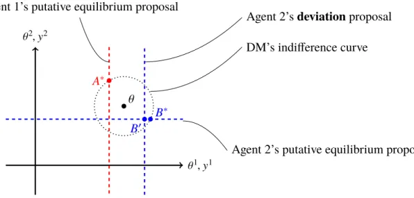
θ¹,y¹ θ²,y²

θ

Agent 1’s putative equilibrium proposal

Agent 2’s putative equilibrium proposal Agent 2’sdeviationproposal

A^∗

B^∗ B⁰

DM’s indifference curve

Figure 1.1: Only vague about misaligned dimensions

This mechanism through which competition shapes information revelation can be used to gain insights into electoral competition. There is active research on how parties choose which issues to campaign on as well as invest effort in if elected (Ash, Morelli, and Van Weelden, 2015; Egorov, 2015). In the language of this paper, campaign issue choice is a way for informed political parties to make policy commitments and I draw a connection between this choice and parties’ interest alignment with voters. This paper is also related to ambiguity in political campaigns (Meirowitz, 2005; Alesina and Holden, 2008; Kamada and Sugaya, 2014; Kartik, Van Weelden, and Wolton, 2015). This literature focuses on the existence of vagueness when the state space is one-dimensional, whereas I study a multidimensional state space and where vagueness occurs.

An Example

To see why it may be unwise to commit to a specific action, consider a DM choosing an agent to make a two-dimensional decisiony = (y¹,y²). I refer to the vectorθ−y as the outcome, whereθ ∈ R²is the state of the world that is unknown to the DM but known to the two agents. All players have quadratic utilities characterized by their ideal actions given the state. Figure 1.1 illustrates players’ ideal actions for any given stateθ. The DM’s ideal action equalsθ. Each agent has a constant bias.

A^∗ and B^∗ are Agent 1 and Agent 2’s ideal actions given θ, respectively. Note that the horizontal distance between A^∗ and θ is smaller than that between B^∗ and θ, and the vertical distance between B^∗ andθ is smaller than that between A^∗ and θ. Dimension 1 is then called Agent 1’saligned dimensionand Agent 2’smisaligned

(12)

dimension. The opposite is true for dimension 2.

Consider the putative equilibrium proposals by the agents as shown in Figure 1.1.

Agenti’s proposal has a specific commitment to his ideal action on dimensioni, but is vague about dimension j. Since he is free to implement any action for dimension j if chosen, the rational choice is to implement his ideal action. So overall he will choose his ideal action on each dimension. Since A^∗ and B^∗ are of equal distance toθ, the DM is indifferent between agents’ ideal actions and assumed to randomize 50-50 between the agents. Lastly, notice that since each agent commits on his ideal action on dimensioni, the DM learnsθⁱ from Agenti.

However, either agent has an incentive to deviate. Suppose that Agent 2 deviates as follows: instead of being vague about his misaligned dimension, now he is vague about his aligned dimension. The DM is surprised by the proposal profile she observes and her belief over Θ is unspecified. Moreover, for some beliefs, she prefers Agent 2 while the opposite is true for other beliefs. The key to decide which agent is better is to determine the sensible beliefs.

The key idea is that when Agent 2 deviates to make a surprising proposal, the DM should still believe in the information content of Agent 1’s proposal. That is, she should believe that Agent 1 has not deviated and learns θ¹ from his proposal.

Given this belief, which agent is better? Agent 2 is compromising on dimension 1 by committing to a less biased action. For dimension 2, since he is vague he implements his ideal action. So B⁰ is the action Agent 2 has deviated to. As in equilibrium, Agent 1 will implement A^∗. The DM then strictly prefers Agent 2.

Since in equilibrium Agent 2 gets A^∗half the time andB^∗half the time, Agent 2 has made a profitable deviation.

Hence, revealing the state for the opponent’s misaligned dimension creates a visible target for him to react to. Vagueness, however, allows the DM’s belief to create an insurmountable obstacle for the opponent. Suppose instead that in equilibrium, Agent 1 is vague about both dimensions. Then any concession by Agent 2 is incredible, since nothing stops the DM from believing that he is proposing his own ideal action. For convenience, here I focus on a special case in which no agents have an overall advantage. In Section 1.3, I discuss a general-bias case while still retaining the feature that each agent has a advantage over a dimension. I also provide conditions for the existence of equilibria in which agents are vague about their aligned dimensions only.

(13)

Relation to Existing Literature

To my knowledge, this is the first paper to address competition for delegation in a multidimensional action and state space. Ambrus, Baranovskyi, and Kolb (2015), the first study of competition for delegation, uses a one-dimensional setup.

Battaglini (2002) studies a multidimensional setting, but communication takes the form of cheap talk. Neither studies the role of vagueness in information disclosure.

My paper is connected to the disclosure literature (see Dranove and Jin (2010) for a survey). Here I briefly discuss the connection of my paper with Grossman (1981).

He studies an environment in which a seller chooses whether to credibly disclose his quality and shows that all types of sellers fully disclose. The idea is that suppose two sellers of different qualities are pooled together. Then the buyer is only willing to pay the price as if the quality is an average of the two. Now the higher-quality of the two sellers can profit by disclosing his quality and receive a higher price, since the buyer now has a higher willingness to pay. The argument is based on the assumption that the seller could always have disclosed his exact quality. The counterpart of exact disclosure in my model is vagueness. An agent can always be vague and let the DM know the payoff from choosing him. The difference is that vagueness serves an additional purpose, which is masking the state of the world.

This helps sustaining vagueness in equilibrium.

This paper is broadly related to work on competition in information revelation, which takes two forms: verifiable information revelation and cheap talk communication. The former (Gul and Pesendorfer, 2012; Gentzkow and Kamenica, 2015) assumes that informed parties cannot distort information; they can only decide how much information to provide. Cheap talk communication with multiple senders is investigated by Krishna and Morgan (2001) and Battaglini (2002). In particular, informativeness of cheap talk in electoral campaigns is studied by Schnakenberg (2014),Kartik, Squintani, and Tinn (2015) and Kartik and Van Weelden (2014).

Blume, O. J. Board, and Kawamura (2007) and Blume and O. Board (2014) study vagueness in one-sender cheap talk in the form of noisy messages.

Another strand of related literature is delegation to informed, biased agents. Alonso and Matouschek (2008) study the DM’s problem of how to optimally restrict the set of actions that an agent can take. Li and Suen (2004) discuss when a DM should delegate, and how biased the agent should be in order to be delegated. I focus on the communication from agent to the DM and assume that the only choice the DM can make is choosing between two agents. Ambrus, Baranovskyi, and Kolb

(14)

(2015)’s question is probably closest to mine. They investigate agents’ proposals when a coarsely informed DM lacks the ability to measure the difference between two proposed actions. They demonstrate the existence of equilibrium in which agents distort their private signals. Distortion comes from the fact that the agents are imperfectly informed, while I study perfectly informed agents.

Lastly, this paper contributes to the equilibrium refinement literature. Refinement for one-sender signaling games is well-studied (Cho and Kreps, 1987; Banks and Sobel, 1987). Vida and Honryo (2015) study the implication of strategic stability (Kohlberg and Mertens, 1986) in general multi-sender signaling games. They find that stability implies a condition for out-of-equilibrium beliefs which states that the receiver rationalizes an out-of-equilibrium signal with the minimal number of deviations (Bagwell and Ramey, 1991). Schultz (1996) applies this belief restriction in a game where two informed parties decide how much public good to provide.

1.2 The Model

A decision affecting a decision maker (DM) and two agents needs to be made.

The DM is unable to implement actions and has to delegate it to one of the two agents. Only the agents have the relevant information that pertains to the decision making — they observe a state of the world that determines the consequence of any given action. Afterwards, agents simultaneously announce proposals. The DM then chooses an agent to implement his proposal.

The state, denoted by θ = (θ¹, θ²), concerns two dimensions: θ¹ is the state on dimension 1 andθ²on dimension 2. θis distributed overΘ≡R²according to some continuous distribution function F with density f. f has full support onR². The space of proposals is M = (R∪ {∅})², whereRis the action space and ∅denotes a message indicating vagueness. For i = 1,2, mi = (m_i¹,m²_i) denotes Agent i’s proposal andm= (m₁,m₂)denotes the proposal profile.

If Agentiis chosen, he implements an actionyi = (y_i¹,y_i²) ∈R². For each dimension k ∈ {1,2}, the set of feasible actions depends onm_i^k as follows. If Agentiis specific about dimension k and announces m_i^k ∈ R, then he is committed to m_i^k and must choose y_i^k = m_i^k. If Agenti is vague about dimension k and announces m_i^k = ∅, then he is free to choose any actiony_i^k ∈R.

The DM and the agents have conflicting interests. When the state isθand the action isy, the DM’s payoff is

ud(θ,y)= −(θ¹−y¹)²−(θ²− y²)².

(15)

Agent 1 and 2’s payoffs are

u₁(θ,y) =−(θ¹−y¹−b¹

1)²−(θ²− y²−b²

1)², u₂(θ,y) =−(θ¹−y¹−b¹₂)²−(θ²− y²−b²₂)², whereb₁= (b¹

1,b²

1)andb₂ = (b¹

2,b²

2)are agents’ biases. Given the stateθ, the DM’s ideal action equals to the state. Agenti’s ideal action is equal toθ−bi. Throughout the paper I assume that|b¹

1|< |b¹

2|and|b²

2|< |b²

1|. Since for dimension 1 Agent 1 is less biased than Agent 2, I call dimension 1 Agent 1’saligned dimensionand Agent 2’s misaligned dimension. The opposite is true for dimension 2. The rule of the game, all players’ utility functions (and therefore their ideal actions given the state), and the state distribution are common knowledge.

An agent’s proposal is sufficient for the DM to evaluate her expected payoff from choosing him. To see this, note that if an agent is specific on a dimension, he implements his proposed action. If he is vague on a dimension, he rationally takes his ideal action contingent on the state observed. Since the DM knows the biases of agents, her payoff from choosing this agent is also fixed. Therefore we can ignore agents’ eventual action choices and focus on their proposals. A pure strategy for Agent i is a function si : Θ → M mapping states into proposals. A strategy for the DM is a function β : M × M → [0,1] mapping proposal profiles into the probabilities that Agent 1 is chosen. The DM’s posterior belief µ: M×M →∆(Θ) maps each possible proposal profileminto a probability measure µ(· | m)overΘ. I use the solution concept of weak perfect Bayesian equilibrium (weak PBE) (s₁,s₂, β, µ) satisfying single-deviation consistency. This new consistency notion limits how the DM updates her belief about agents’ strategies when she is surprised.

After observing a surprising move by the agents, she updates her belief under the assumption that agents make strategic choices independently. As a result, knowing that one agent has deviated does not impact her belief about the other agent’s strategy. To simplify the analysis, I focus on equilibria in which agents play pure strategies on the equilibrium path, the DM randomizes 50−50 whenever indifferent, agents’ choices of vagueness do not depend on the state realization (the invariance condition) and are symmetric (the symmetry condition). The invariance condition says that if Agenti is vague (specific) about dimension k at some state θ, then he is vague (specific) about dimension k at all states. The symmetry condition says that if Agenti is vague about his misaligned (aligned) dimension, then Agent j is also vague about his misaligned (aligned) dimension, which is Agent i’s aligned (misaligned) dimension. Therefore two agents’ choices of vagueness depend on

(16)

their comparative advantage in the same way. Note that I do not assume agents play symmetric strategies, only that the choice of vagueness is symmetric. Agents can vary their specific proposals differently according to the state. From now on, a weak PBE satisfying above requirements is abbreviated as “an equilibrium.” An equilibrium with vagueness is one in which vagueness is supported in equilibrium on some dimension by some agent.

Before formally defining the equilibrium, I first define single-deviation consistency.

Given a weak PBE(s₁,s₂, β, µ), the priorF ∈∆(Θ)induces a probability distribu- tionG₁ ∈∆(M) throughs₁,G₂ ∈ ∆(M)throughs₂, andG₀ ∈ ∆(M ×M)through s₁and s₂. Letsupp(Gk) denote the support ofGk, k = 0, 1, 2. Agenti’s proposal mi isconsistent with equilibriumifmi ∈ supp(Gi),inconsistent with equilibriumif otherwise. A proposal profilemison-pathifm ∈supp(G₀),off-pathif otherwise.

Definition 1 (Single-deviation consistency) Let(s₁,s₂, β, µ) be a weak PBE and F ∈∆(Θ)the prior which inducesG₁,G₂ ∈∆(M)andG₀ ∈∆(M×M). The DM’s belief µsatisfies single-deviation consistency if, for allm = (m₁,m₂)< supp(G₀),

µ(m) ∈∆({θ ∈Θ |s₁(θ)= m₁} ∪ {θ ∈Θ | s₂(θ) =m₂})

when {θ ∈ Θ | s₁(θ) = m₁} ∪ {θ ∈ Θ | s₂(θ) = m₂} is nonempty. Otherwise µ(m) ∈∆(Θ).

In other words, a DM faced with an off-path(m₁,m₂)believes that either Agent 1 or Agent 2 has not deviated whenever believing so is possible.

To understand the definition, let’s divide the possible off-pathm = (m₁,m₂)into the following cases:

1. Neitherm₁orm₂is consistent with equilibrium;

2. miis consistent with equilibrium butmj is inconsistent with equilibrium;

3. Bothm₁andm₂are consistent with equilibrium;

In Case 1, the DM learns that both agents have deviated. Since neitherm₁norm₂is consistent with equilibrium, both {θ ∈ Θ | s₁(θ) = m₁}and {θ ∈ Θ | s₂(θ) = m₂} are empty sets and µ(m)is unrestricted according to Definition 1. Since the DM’s action following a bilateral deviation is irrelevant in sustaining the equilibrium, so is her belief.

(17)

In Case 2, only Agent j is inconsistent with equilibrium. The DM learns that Agent j has deviated. But the DM has the freedom to either believe that Agent i has also deviated or that Agent i is playing according to equilibrium. Since {θ ∈ Θ | si(θ) = mi} is nonempty while{θ ∈ Θ | sj(θ) = mj} is empty, the DM believes that Agentihas not deviated.

In Case 3, both agents are consistent with equilibrium. To see how this can be possible for an off-pathm, consider a putative equilibrium in whichs₁(θ) = s₂(θ) = θ for all θ. Now suppose that at some state θ, Agent 1 deviates to the proposal m⁰

1 = θ , θ. The DM then observes a proposal profile (θ, θ). This is an off-path proposal profile because in equilibrium agents announce the same proposal. Since m is off-path, by definition at noθ are s₁(θ) = m₁ and s₂(θ) = m₂both satisfied.

So at least one agent has deviated. In other words, if the DM believes that Agent 1 has not deviated, then she believes that Agent 2 has deviated; if she believes that Agent 2 has not deviated, then she believes that Agent 1 has deviated. Since both {θ ∈ Θ | si(θ) = mi} and {θ ∈ Θ | sj(θ) = mj} are nonempty, she can indeed believe that Agent 1 has not deviated (and so Agent 2 has deviated), or that Agent 2 has not deviated (and so Agent 1 has deviated). Since she cannot decide who the deviator is, her belief allows both cases.

To summarize, for all possible off-path proposal profiles that the DM may face following a unilateral deviation of an agent, the DM identifies the deviator according to single-deviation consistency. It is important to identify the deviator and non- deviator because the DM can rely on the information contained in the non-deviator’s proposal and his equilibrium strategy to infer the state.

The notion of single-deviation consistency applies to general signaling games. Its intuition is as follows. If the DM believes that agents make independent strategic choices, then whether an agent has deviated should depend on that agent’s proposal only and not his opponent’s. Suppose that Agentiis inconsistent with equilibrium while Agent j is consistent with equilibrium. The DM learns that Agent i has deviated, but she should not use this fact as an excuse to change her belief about Agent j’s strategy. She should continue to believe that Agent j is playing his equilibrium strategy sj. The single-deviation consistency shuts down the channel in which one agent’s deviation impacts the DM’s belief about the other agent. On the other hand, suppose that both agents are consistent with equilibrium. The single-deviation consistency implies that the DM imposes minimal departure from rationality to rationalize deviations and believes that only one agent is the deviator

(18)

whenever possible.

The notion that agents’ strategic choices are independent is not new. Battigalli (1996) defines the independence property for conditional systems over the strategy profiles.

An implication of independence is that the marginal conditional probabilities about player i’s strategies are independent of information which exclusively concerns player j’s strategies. It is shown that the independence property of conditional systems is necessary for an equivalent assessment to satisfy the consistency notion of sequential equilibrium (Kreps and Wilson, 1982).

Watson (2015) first formally defines perfect Bayesian equilibrium for infinite games without nature moves. The definition retains sequential rationality and puts forward a new notion for consistency, called “plain consistency.” Under this framework, the DM’s belief has two components: her belief over the strategies of agents and over the state. Since the latter is determined by the former and the proposal profile observed, we can focus on the belief over strategies. According to plain consistency, the DM assigns probability 1 to Agents playing their equilibrium strategies. When she reaches an off-pathm= (m₁,m₂)wherem₂is inconsistent with equilibrium and m₁is consistent with equilibrium, she only alters her belief about Agent 2’s strategy.

Her belief about Agent 1 should remain as before and so concentrate on Agent 1’s equilibrium strategy.

Now we have all the ingredients for the equilibrium definition:

Definition 2 (Equilibrium) An equilibrium(s₁,s₂, β, µ)is a weak PBE in which 1. si :Θ→ M,i= 1,2;

2. β : M× M → {0,¹

2,1};

3. µsatisfies single-deviation consistency;

4. (Invariance) Fori ∈ {1,2}andk ∈ {1,2},

a) ifs_i^k(θ)= ∅for someθ, thens_i^k(θ)= ∅for allθ;

b) ifs_i^k(θ), ∅for someθ, thens_i^k(θ), ∅for allθ.

5. (Symmetry)∀θ,

a) ifs₁(θ) = (∅,∅), thens₂(θ)= (∅,∅);

b) ifs₁(θ) = (∅,w)for somew ∈R, thens₂(θ)= (z,∅)for somez ∈R;

(19)

c) ifs₁(θ) = (w,∅)for somew ∈R, thens₂(θ)= (∅,z)for somez ∈R; Just to clarify, 4 and 5 are conditions on agents’ equilibrium strategies, not the set of proposals that agents can deviate to. In particular, at any state, an agent is free to deviate to a proposal that is vague about any dimension regardless of his bias and the state realization. I investigate the consequence of dropping the symmetry condition in a smaller state space in Appendix II.

1.3 Main Results

What should agents be vague about? Common wisdom may suggest that agents should focus on the dimension that they have advantages on and ignore others. As a result, an agent should commit on their aligned dimension and be vague about their misaligned dimension. The model suggests otherwise. If Agent 1 is vague about dimension 1, then being vague is beneficial since the DM already trusts him on this dimension. More importantly, for any commitment made by Agent 2, the DM is free to believe that Agent 2 is committing on his own ideal action since she has arrived at an off-path information set. On the other hand, if Agent 1 is specific about dimension 1 and reveals θ¹ to the DM, Agent 2 can anchor on this revealed information and deviates by offering a compromise. The DM believes that only Agent 2 has deviated and continues to trust the information aboutθ¹revealed by Agent 1. This way Agent 2 is able to credibly compromise on his misaligned dimension.

The results characterize equilibria in terms of where vagueness occurs in agents’

proposals and construct an equilibrium. I first consider the case in which agents have zero biases on their aligned dimensions.

Proposition 1 Suppose thatb¹

1 = b²

2 = 0. In all equilibria with vagueness, vague- ness occurs on agents’ aligned dimensions. An equilibrium in which vagueness only occurs on agents’ aligned dimensions exists.

All proofs are relegated to Appendix I. Here I demonstrate the intuition behind the proof. By Definition 2, in any equilibrium with vagueness, the agents’ proposal profile must take one of the following forms:

1. s₁(θ)= s₂(θ)= (∅,∅),∀θ.

2. s₁(θ) ∈ {∅} ×R, s₂(θ) ∈R× {∅},∀θ.

(20)

3. s₁(θ) ∈R× {∅}, s₂(θ) ∈ {∅} ×R,∀θ.

In both 1 and 2, vagueness occurs on agents’ aligned dimensions. In 3, vagueness only occurs on agents’ misaligned dimensions. I show that 3 cannot be an equilibrium proposal profile. Suppose first that both agents commit to their ideal actions on their aligned dimensions. The DM then learnsθⁱ from Agenti,i = 1, 2. Now suppose that some Agentideviates to compromise on his misaligned dimension, i.e.

propose an action preferred by the DM to his ideal action. By single-deviation consistency, the DM continues to believe the information revealed bymjand therefore realizes that Agentiis making a compromise. This deviation is profitable as long as the compromise is small enough. The rest of the argument establishes that agents commit to their ideal actions on their aligned dimensions given that they have zero bias.

Although agents cannot be vague only about their misaligned dimensions, they can be vague only about their aligned dimensions. Consider the following putative equilibrium proposals for the agents: s^∗

1(θ) = (∅, θ²−b²

1),s^∗

2(θ) = (θ¹−b¹

2,∅) for allθ. In this equilibrium, each agent reveals the state for his misaligned dimension and implements his ideal action on each dimension. Consider a potential deviation by Agentito make compromises on dimensioniand propose an action strictly better for the DM than his ideal action. This deviation leads to an on-path proposal profile and the DM chooses his equilibrium action. Since Agentideviates to a worse action but retains his equilibrium probability of winning, the deviation is unprofitable. The rest of the argument shows that even if an agent deviates to a compromise which is inconsistent with equilibrium (so that the DM realizes that he has deviated), the DM is free to believe that his action is his own ideal action and will not change his probability of winning.

Proposition 1 characterizes equilibria with vagueness and establishes its existence when agents have zero biases on their aligned dimensions. The next proposition does so under a more general bias structure and illustrates that the undercutting intuition still applies. With arbitrary bias, it is hard to demonstrate that the equilibrium proposals must be fully revealing regarding the dimension that it is specific about.

However, starting with a fully-revealing equilibrium such as one in the following, it is easy to see that such strategies cannot be sustained in equilibrium.

Proposition 2 Suppose that |b¹

1|< |b¹

2| and |b²

2|< |b²

1|. Then both agents commit- ting to their ideal actions on the aligned dimensions and being vague about their

(21)

misaligned dimensions cannot be sustained in equilibrium. Both agents being vague about both dimensions can be sustained in equilibrium.

Consider a putative equilibrium proposal profile in which both agents are vague about all dimensions in all states: s^∗

1(θ) = s^∗

2(θ) = (∅,∅),∀θ. Suppose at someθ, Agent 1 deviates to be specific about any given dimension(s). The deviation leads to an off-path proposal profile, at which point the DM should maintain the belief that Agent 2 has not deviated but is free to choose any beliefs regarding Agent 1’s strategy. One of the beliefs that can deter this deviation and therefore support (s^∗

1, s^∗

2) as part of an equilibrium is the belief that Agent 1 has deviated to his own ideal action. Under this belief, the DM maintains his equilibrium action. Since Agent 1’s deviation action cannot be strictly preferred to his own ideal action and he gets the same probability of winning as in equilibrium, such a deviation is unprofitable.

1.4 Refinement: Extended Intuitive Criterion

In the last section, I showed that there exist equilibria in which agents are vague about their aligned dimensions. But this should not come as a surprise. In signaling games, there typically exist multiple equilibria supported by unreasonable beliefs. In this section, I show that the beliefs supporting the equilibria I identified are actually very reasonable in the sense that they satisfy a refinement similar to the Intuitive Criterion, adapted for two-sender games. The refinement combines the Intuitive Criterion for one-sender games with single-deviation consistency. For an off-path proposal profile, single-deviation consistency identifies the deviator. The Intuitive Criterion restricts what types of deviations the DM is allowed to believe in.

One-sender: Intuitive Criterion

The Intuitive Criterion for one-sender signaling games places restrictions on the receiver’s beliefs after an unexpected message by the sender. The receiver is required to believe that the sender’s private information is such that the highest payoff that the sender can get by deviating to the observed message is weakly higher than the sender’s equilibrium payoff, given that the receiver does not react to the message with dominated actions.

First I review the idea of Intuitive Criterion. For consistency, I will keep using the terminologies and notations from Section 2.2 to describe both one-sender and two- sender signaling games and the equilibrium refinements. In a one-sender signaling game, given the state θ, the Agent’s proposal m ∈ M, the DM’s action β ∈ B, the

(22)

Agent’s utility is denoted byua(θ,m, β)and the DM’s utilityud(θ,m, β). The DM’s belief overΘgiven mis denoted by µ(· | m). Givenm and µ, the set of the DM’s best responses is:

BRg(µ,m) =arg max

β∈B

Z

Θ

ud(θ,m, β) dµ(θ | m).

For any nonemptyT ⊂ Θandm∈ M, BR(T,m) = [

µ:µ(T|m)=1

BRg(µ,m)

denotes the set of the DM’s best responses according to beliefs supported on T. WhenT is empty, let BR(T,m) =BR(Θ,m).

Given an equilibrium(s^∗, β^∗, µ^∗), the Agent’s equilibrium payoff at θis denoted by u^∗_a(θ). For an off-path proposal m⁰, the set of states at which the Agent’s highest payoff from deviating tom⁰given that the DM best responds to some belief is higher than the Agent’s equilibrium payoff is

Θ(m⁰) = {θ | max

β∈BR(Θ,m⁰)ua(θ,m⁰, β) ≥ u^∗_a(θ)}.

Finally, an equilibrium(s^∗, β^∗, µ^∗) fails the Intuitive Criterionif there existsθ ∈Θ and off-pathm⁰∈ M such that

u^∗_a(θ) < min

β∈BR(^Θ(m⁰^),m⁰)ua(θ,m⁰, β).

When the DM observes an unexpected proposal m⁰, the support of her belief is restricted to be states at whichm⁰is potentially profitable. That is, the highest payoff that the Agent can get given that the DM does not play dominated actions is weakly higher than his equilibrium payoff. The Agent then contemplates deviations given that the DM best responds to beliefs thus restricted. If for some θ and off-path proposalm⁰, any such best response makes the Agent strictly better off compared to in equilibrium when the state isθ, then the equilibrium fails the Intuitive Criterion.

Two-sender: Extended Intuitive Criterion

I extend the Intuitive Criterion to the two-sender case by combining single-deviation consistency with the Intuitive Criterion. Single-deviation consistency identifies the deviator. The Intuitive Criterion identifies the kind of deviations that the receiver is allowed to believe in.

In a two-sender signaling game, given the state θ ∈ Θ, agents’ proposal profile m = (m₁,m₂), and the DM’s action β ∈ B, Agenti’s utility is denoted byui(θ,m, β) and the DM’s utilityud(θ,m, β)wherem= (m₁,m₂). Letµ(· | m)denote the DM’s belief over Θ conditional on m. Given an equilibrium (s^∗

1,s^∗

2, β^∗, µ^∗), Agent i’s

(23)

equilibrium payoff atθis denoted byu_i^∗(θ). Similar as before,G₀is the distribution overM×M induced by the equilibrium strategies (s^∗

1, s^∗

2) and the state distribution F over Θ. Gi (i = 1,2) is the distribution over M induced by s^∗_i and F. I now introduce the equilibrium refinement.

Definition 3 (The Extended Intuitive Criterion) Let (s^∗

1,s^∗

2, β^∗, µ^∗) be a weak PBE of a two-sender signaling game. For each m = (m₁,m₂) < supp(G₀) and i ∈1,2, form the set

Θ_i(m) = (

θ | s^∗_j(θ)= mj,u^∗_i(θ) ≤ max

β∈BR(Θ,m)ui(θ,sj(θ),mi, β) )

. (s^∗

1,s^∗

2, β^∗, µ^∗)fails the Extended Intuitive Criterion if there existsθ ∈Θ,i ∈ {1,2}, m⁰_i ∈ Msuch that

u^∗_i(θ) < min

β∈BR(^Θ1(m⁰)∪Θ₂(m⁰),m⁰)ui(θ,m⁰, β),

where m⁰= (m_i⁰,sj(θ)). An equilibrium satisfying the Extended Intuitive Criterion is called an intuitive equilibrium.

Whenever the DM faces an off-path proposal profile m⁰, her belief is restricted to be supported on Θ₁(m⁰) ∪Θ₂(m⁰). Θ_i(m⁰) is the set of states at which only Agenti is the deviator and his deviation is potentially profitable. In calculating the payoff from deviating, apart from assuming that the DM does not play dominated actions, the Agent also assumes that the other Agent plays according to equilibrium.

Note that Θ_i(m) may be empty because mj < supp(Gj) or mi is not potentially profitable. However, as long as m results from a unilateral deviation and the deviation is potentially profitable, Θ₁(m)∪Θ₂(m) is nonempty. An equilibrium fails the Extended Intuitive Criterion if at some stateθ, some Agentican profitably deviate to some m⁰_i as long as the DM best responds to restricted beliefs upon observing(m⁰_i,sj(θ)).

Robustness of Equilibria

Previously I have identified some equilibria in which agents are vague about their aligned dimensions. When|b¹

1|< |b¹

2|and|b²

2|< |b²

1|, s₁(θ) = s₂(θ) = (∅,∅),∀θ can be sustained in equilibrium. As a special case, whenb¹

1 = b²

2 =0 s₁(θ) = (∅, θ²−b²₁),s₂(θ) = (θ¹−b¹₂,∅),∀θ

can also be sustained in equilibrium. As it turns out, both of them are robust to the Extended Intuitive Criterion refinement.

(24)

Proposition 3 Suppose that|b¹

1|< |b¹

2|and|b²

2|< |b¹

2|. Intuitive equilibria in which both agents are vague about their aligned dimensions exist. Furthermore if b¹

1 = b²

2 = 0, in all intuitive equilibria with vagueness, vagueness occurs on agents’

aligned dimensions.

The equilibrium in which both agents are vague about both dimensions is supported by the following belief: whenever one of the agents deviates, he is committing to his own ideal action for the dimensions he is specific about. To show that this belief satisfies single-deviation consistency, I first show that for some β ∈ {0,¹

2,1}, committing to own ideal action gives the deviator higher payoff compared to equilibrium. Then I show that there is some belief µ∈∆(Θ)according to which

β is a best response, and hence β is not dominated.

Furthermore when b¹

1 = b²

2 = 0, I show that the putative equilibria in which both agents are only vague about their misaligned dimensions do not satisfy the Extended Intuitive Criterion. In fact, if we require the DM’s belief to satisfy single-deviation consistency, then any agent has a profitable deviation. For this deviation, all the beliefs satisfying single-deviation consistency in fact concentrate on the event that the deviator has made a potentially profitable deviation. Essentially, the Extended Intuitive Criterion does not put further restriction on beliefs apart from those imposed by single-deviation consistency. So the equilibria in which agents are only vague about their misaligned dimensions are not intuitive equilibria. This establishes that all the intuitive equilibria with vagueness has vagueness occurring on agents’

aligned dimensions.

1.5 Discussion

One may be interested in knowing how allowing agents’ vagueness impacts the DM’s payoff. To illustrate this, consider a game which is identical to the setup so far except that agents are not allowed to be vague. That is, M = R². There are two consequences of such a restriction. First, it is hard to sustain a simple fully-revealing equilibrium. For example, consider a putative equilibrium in which s₁(θ) = s₂(θ) =θ, for allθ. This is in fact not a weak PBE because at anyθ ∈R², there is ˜θ ∈R²such that exactly one of the two following events happens: either ˜θ is a profitable deviation for Agent 1 atθ, orθ is a profitable deviation for Agent 2 at ˜θ. The key reason is, whenever an agent deviates, the DM cannot tell who the deviator is. Therefore she must take the same action after seeing Agent 1 proposes θ˜and Agent 2 proposesθ. If her action is favorable towards Agent 1, then Agent 1

(25)

has an incentive to deviate; otherwise Agent 2 has an incentive to deviate.

Second, the DM can potentially get worse-off due to not allowing agents’ vagueness.

To see this, consider the following equilibrium: s₁(θ) = s₂(θ) = (θ¹, θ²) for all θ. The reason that both agents making the same constant proposal can be sustained in equilibrium is that, whenever an agent deviates to an alternative action on either dimension, the DM is free to believe that the optimal action is closer to the equilibrium action than the deviator’s action. In this equilibrium, the DM gets a payoff that depends on the distance from the state realization and the equilibrium proposal.

Consider a pooling equilibrium in the with-vagueness setup: s₁(θ) = s₂(θ) = (∅,∅) for allθ. This equilibrium is very similar to the constant equilibrium above since it is also supported by the belief that any deviation is no better than equilibrium for the DM. However in this equilibrium, the DM gets the less-biased agent’s ideal action.

If his bias is sufficiently small, then the all-vague equilibrium is better for the DM.

This is the case because when agents are always vague, undercutting is essentially ruled out. Therefore agents can secure their ideal actions without worrying that their opponent will offer a more favorable action to the DM. The undercutting leads to an equilibrium in which both agents offer the optimal action, which turns out to be non-equilibrium as shown above. Vagueness protects agents from making concessions that lead to non-existence of equilibrium.

Appendix I.

Throughout the proof, I useu_i^dev(θ,m_i^dev,mj)to denote Agenti’s payoff after deviating tom^dev_i at stateθ, at which Agent j’s equilibrium proposal ismj. πidenotes the DM’s expected payoff from choosing Agentigiven her beliefs and agents’ proposals.

Given Agenti’s proposalmi, yi(mi) denotes Agenti’s policy. u^∗_i(θ)denotes Agent i’s equilibrium payoff at stateθ.

Lemma 1 Suppose that the agents’ strategiess₁,s₂are as follows:

s₁(θ)= (w(θ),∅), s₂(θ)= (∅,z(θ)), wherew,z :Θ→R. Then β(s₁(θ),s₂(θ))= ¹₂for allθ.

(26)

Proof. Suppose that β(s₁(θ),s₂(θ)) = 0 for someθ. Then Agent 1 has a profitable deviations₂(θ). To see this, first note that Agent 1’s equilibrium payoff atθ is

u^∗

1(θ) =u₁(θ,y₂(∅,z(θ))) =u₁((θ¹, θ²),(θ¹−b¹

2,z(θ))).

Now let Agent 1 deviate tos₂(θ). Givenm= (m^dev

1 ,s₂(θ)) = ((∅,z(θ)),(∅,z(θ))) and anyµ∈∆(Θ),π₁ > π₂. This is because |b¹

1|< |b¹

2|and both agents propose the same action on dimension 2. Therefore β(m) =1 and Agent 1’s deviation payoff is

u^dev

1 (θ,m^dev

1 ,s₂(θ))= u₁(θ,y₁(∅,z(θ))) =u₁((θ¹, θ²),(θ¹−b¹₁,z(θ))) >u^∗₁(θ).

Similarly, if β(s₁(θ),s₂(θ)) =1 for someθ, then Agent 2 has a profitable deviation s₁(θ). To summarize, agents win with equal probability in equilibrium.

Proof of Proposition 1

The first part of the proof rules out agents’ strategiess₁, s₂as follows:

s₁(θ)= (w(θ),∅), s₂(θ)= (∅,z(θ)),

wherew, z : Θ → R. I prove this by contradiction by first characterizing wand z and then demonstrating incentives to deviate. Without loss of generality, I assume thatb₁= (0,b²

1)andb₂ = (b¹

2,0)wherekb₁k≤ kb₂k. Step 1. β(s₁(θ),s₂(θ))= ¹₂ for allθ.

This follows from Lemma 1.

Step 2. w(θ) =θ¹,z(θ)= θ²,∀θ.

Suppose thatw(θ) ,θ¹for someθ. Then Agent 1 has a profitable deviation(∅,∅). To see this, first note that

u^∗

1(θ)= 1

2u₁(θ,y₁(w(θ),∅))+ 1

2u₁(θ,y₂(∅,z(θ))) < 1

2u₁(θ,y₂(∅,z(θ))).

Now let Agent 1 deviate to m^dev

1 = (∅,∅). Given m = (m^dev

1 ,s₂(θ)) = ((∅,∅),(∅,z(θ))) andµ∈∆(Θ),

π₁ =Z

Θ

ud(θ, θ−b₁)µdθ =−kb₁k², π₂ =

Z

Θ

ud(θ,(θ¹−b¹₂,z(θ))µdθ ≤ Z

Θ

ud(θ,(θ¹−b¹₂, θ²)µdθ = −kb₂k²≤ π₁. Therefore β(m) ≥ ¹

2. Moreover, because for anyθandz(θ), u₁(θ,y₁(∅,∅)) >u₁(θ,y₂(∅,z(θ))),

(27)

we have u^dev

1 (θ,m^dev

1 ,s₂(θ)) ≥ 1 2

u₁(θ,y₁(∅,∅))+ 1 2

u₁(θ,y₂(∅,z(θ)))

= 1

2u₁(θ,y₂(∅,z(θ)))

>u^∗₁(θ).

(∅,∅) is then a profitable deviation for Agent 1. Therefore w(θ) = θ¹ for all θ and π₁ = −kb₁k². Since β(s₁(θ),s₂(θ)) = ¹₂ for all θ, π₂ = π₁ = −kb₁k². This immediately rules out kb₁k< kb₂ksince

π₂= Z

Θ

ud(θ,(θ¹−b¹

2,z))µdθ ≤ Z

Θ

ud(θ,(θ¹−b¹

2, θ²))µdθ =−kb₂k²< −kb₁k². Therefore s₁, s₂ can only be sustained in equilibrium when kb₁k= kb₂k. In this case, I use the same argument as above to show z(θ) =θ²for allθ.

We have finished characterizingwandz. Given thatw(θ) = θ¹,z(θ) = θ², for allθ, u₁^∗(θ) = 1

2u₁(θ, θ−b₁)+ 1

2u₁(θ, θ−b₂)= −1 2

kb₁−b₂k². Step 3. At anyθ, Agent 1 has a profitable deviation(∅, θ²−(1−)b²

1), where > 0 is small.

Suppose that Agent 1 deviates to said proposal at θ. The DM observes m = (m^dev

1 ,s₂(θ)) = ((∅, θ² − (1− )b²

1),(∅, θ²)) and believes that only Agent 1 has deviated. Therefore µ(m) ∈∆(T(m)), where

T(m) = {θ | s₂(θ) = (∅, θ²)} ={θ | θ²= θ²}.

For any µ∈∆(T(m)), π₂=

Z

Θ

ud(θ, θ−b₂)µdθ =−kb₂k²=−kb₁k², π₁= Z

Θ

ud(θ,(θ¹, θ²−(1−)b²

1))µd(θ)

= Z

Θ

ud(θ,(θ¹, θ²−1+))µdθ =−k(1−)b₁k²> π₂. Therefore β(m)= 1 and for small enough.

u^dev₁ (θ,m₁^dev,s₁(θ)) =u₁(θ,(θ¹, θ²−(1−)b²₁))= k(0, b²₁)k²=−²(b²₁)²> u^∗₁(θ), making(∅, θ²−(1−)b²

1) a profitable deviation.

The second part of the proof establishes

s₁(θ) = (∅, θ²−b²

1), s₂(θ) = (θ¹−b¹₂,∅),

as an equilibrium. The DM’s belief and strategy are as follows:

(28)

1. For anym= ((∅,w),(z,∅)) wherew,z ∈R, µ(z+b¹

2,w+b²

1) =1.

β(m)=













1

2 ifkb₁k= kb₂k, 0 ifkb₁k> kb₂k, 1 ifkb₁k< kb₂k.

2. For anym = ((∅,∅),(z,∅)) wherez ∈ R, µ{θ˜ | θ˜¹ = z+b¹

2} = 1 and β(m) is same as 1.

3. For anym= ((w,∅),(z,∅)) wherew,z ∈R, µ{θ˜ |θ˜¹= z+b¹

2}=1.

β(m) =













1

2 ifk(z+b¹

2−w,b²

1)k= kb₂k, 0 ifk(z+b¹

2−w,b²

1)k> kb₂k, 1 ifk(z+b¹

2−w,b²

1)k< kb₂k.

4. For any m = ((q,w),(z,∅)) where q, w, z ∈ R, µ{θ˜ | θ˜¹ = z + b¹

2,θ˜² = w+b²

1}= 1.

β(m)=













1

2 ifk(z+b¹

2−q,b²

1)k= kb₂k, 0 ifk(z+b¹

2−q,b²

1)k> kb₂k, 1 ifk(z+b¹

2−q,b²

1)k< kb₂k. 5. For anym= ((∅,w),(∅,∅))wherew ∈R, µ{θ˜ | θ˜² =w+b²

1}= 1 and β(m) is same as 1.

6. For anym= ((∅,w),(∅,z)) wherew,z ∈R, µ{θ˜ |θ˜²= w+b²

1}= 1.

β(m) =













1

2 ifkb₁k= k(b¹

2,w+b²

1− z)k, 0 ifkb₁k> k(b¹

2,w+b²

1−z)k, 1 ifkb₁k< k(b¹

2,w+b²

1−z)k.

7. For anym= ((∅,w),(q,z)) wherew,q, z ∈R, µ(q+b¹

2,w+b²

1) =1.

β(m) =













1

2 ifkb₁k= k(b¹

2,w+b²

1− z)k, 0 ifkb₁k> k(b¹

2,w+b²

1−z)k, 1 ifkb₁k< k(b¹

2,w+b²

1−z)k.

8. For any otherm, µ∈∆(Θ)and β(m) ∈BRg(µ,m).

µ(· | m) satisfies single-deviation consistency for all m. For m as the result of a unilateral deviation by Agentisuch thatmi <supp(Gi), the DM believes that Agent

Three Essays on Information Economics