Mean amplitude of the load spectrum; (b) cycle change. a) Sample autocorrelation function (ACF) of mean amplitude (c) Sample ACF of cycle variation of load history data; (d) PACF pattern of cycle variation of load history data. a) - (e) Initial probability distribution functions of the ARIMA model. a)-(b) Bound forecast and mean forecast compared to the data when updating.
Overview
Most reliability research has focused only on quantifying the natural variability at the input level, and then estimating the uncertainty at the output level via uncertainty propagation [Beran et al., 2006; Maˆıtre et al., 2007; Wojtkiewicz et al., 2001; Probabilistic methods for addressing data uncertainty in engineering problems are also actively pursued, and some recent developments can be found in [Zaman et al., 2010; Sankararaman and Mahadevan , 2011a , 2012b ].
Research objectives
Within the UQ community, three types of activities are pursued to address different aspects of model uncertainty: (1) model calibration [Kennedy and O'Hagan, 2001], which aims to quantify the uncertainty in the estimation of model parameters, (2) ) model validation [Oberkampf and Trucano, 2004; Rebba et al., 2006; Ling and Mahadevan , 2013b ], which is used to quantify the uncertainty and confidence in model prediction, and (3) model verification [ Babuska and Oden , 2004 ; ASME, 2006; Rangavajhala et al., 2011], which focuses on solution approximation error. The fourth task examines methods of incorporating data collected on an in-service system (eg loading data, inspection data) into the reliability analysis.
Organization of the dissertation
It can be observed that the weight of the ARIMA(2,1,0) model increases to almost one in a short time, which means that the ARIMA(2,1,0) model fits the data better. It can be seen from the results that the uncertainty in the forecast for the four scenarios drops significantly after inspection.
BACKGROUND
Brief introduction to Bayesian networks
The conditional probability of Xi given its parent nodes, p(Xi|PaXi), can be found in the conditional probability table. For example, if QoI is in the set ¯Uobs, the posterior probability distribution of QoI can be obtained by marginalizing the joint posterior distribution p( ¯Uobs|Uobs =D) in Eq.
Bayesian model calibration
- Basic methodology
- Bayesian calibration with interval data
- Bayesian calibration with time series data
- Computational issues
If the measurement uncertainty in the experimental inputs is negligible, xD can be treated as a constant. The likelihood function of the parameters can then be estimated based on running the surrogate model several times.

Quantitative model validation techniques
- Hypothesis testing-based methods
- Classical hypothesis testing
- Bayesian hypothesis testing
- Non-hypothesis testing-based methods
- Reliability-based metric
- Area metric-based method
The p-value for a two-tailed t-test (considering both tails of the distribution) can be obtained as It is defined as the probability that the difference (d) between the observed data (YD) and the model prediction (Ym) will be less than a given tolerance limit.
Time-dependent reliability analysis
- Time-dependent reliability analysis with a single perfor-
- Time-dependent reliability analysis with multiple perfor-
Therefore, the area metric in the transformed probability space can be developed as [Ferson et al., 2008]. For devices with a single performance criterion (denoted by y), the limit state function can be expressed as
Surrogate modeling techniques
- Gaussian process interpolation
- Polynomial chaos expansion
Note that the inverse of the covariance matrix ΣT T is needed in the calculation of the likelihood function in Eq. Thus, training data for the GPC surrogate model is needed at the grid points of these integration algorithms.
Summary
Assessment of confidence in the predictions of these methods can be done using model validation [Sargent, 2005]. The uncertainty in the modified Paris law coefficients - C, n and m - can be represented through their probability distributions.
CHALLENGING ISSUES IN BAYESIAN MODEL CALIBRATION
Introduction
In section 3.2.1 we will investigate Bayesian calibration with five different previous formulations of the model discrepancy function: (1) constant, (2) Gaussian random variable with fixed mean and variance, (3) Gaussian random variable with input-dependent mean and variance, ( 4) Gaussian random process with stationary covariance function, and (5) Gaussian random process. First, Bayesian calibration is performed using each of the five options of the model discrepancy function, and five posterior distributions of model parameters and model discrepancy are obtained.
Formulations and selection of model discrepancy in Bayesian calibration 37
- Model discrepancy as a constant bias
- Model discrepancy as i.i.d. Gaussian random vari-
- Model discrepancy as Gaussian random variables
- Model discrepancy as a Gaussian process with sta-
- Model discrepancy as a Gaussian process with non-
- Assessment and combination of calibration results using a
- Reliability-based model validation metric
- Combining the posterior probability distributions of
- Numerical example
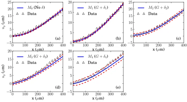
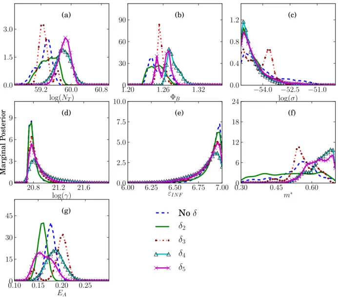
Marginal posterior PDFs of Young's modulus corresponding to different model misfit options are shown in the figure. Thus, when we extrapolate the model from the calibration domain (P = 2.5 µN) to the validation domain (P = 3.5 µN), δ3 and δ4 are no longer good representations of the model discrepancy.
Identifiability of model parameters
The first type of non-identifiability, structural non-identifiability, is due to the redundant parameterization of the model structure. The first case suggests that the model is not identifiable due to the model structure or due to insufficient data.
Calibration of multi-physics computational models
- Integration of multi-physics models and experimental data
- Strategy of Bayesian calibration for multi-physics models . 58
Direct updating of the characteristic matrices is applied to the rain counting method and the Markov chain method. Thus, these three methods can be used to detect the existence of the directional bias.
INTERPRETATIONS, RELATIONSHIPS, AND APPLICATION ISSUES
Introduction
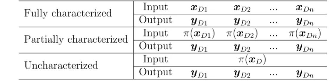
We assume that the same set of variables go into the model and validation experiments as inputs (ie, the terms “model input” and “experimental input” represent the same set of variables), and we compare the results of the model and experiments during validation. While most previous studies focus only on validation with fully characterized experimental data, this chapter explores the use of all three types of data in different validation methods.
Scenarios and decision process of model validation under uncertainty 66
- Interval hypothesis on distribution parameters
- Equality hypothesis on probability density functions
- Bayesian hypothesis testing with multiple data points
With the first formulation, it is straightforward to derive the likelihood functions under the null and alternative hypotheses, and the existence of directional bias can be reflected in the test, as will be shown below. This approach is called "ensemble validation" in this thesis, and the resulting overall Bayes factor in a Bayesian interval/similarity hypothesis test can be calculated as.
Validation with fully characterized, partially characterized, or un-
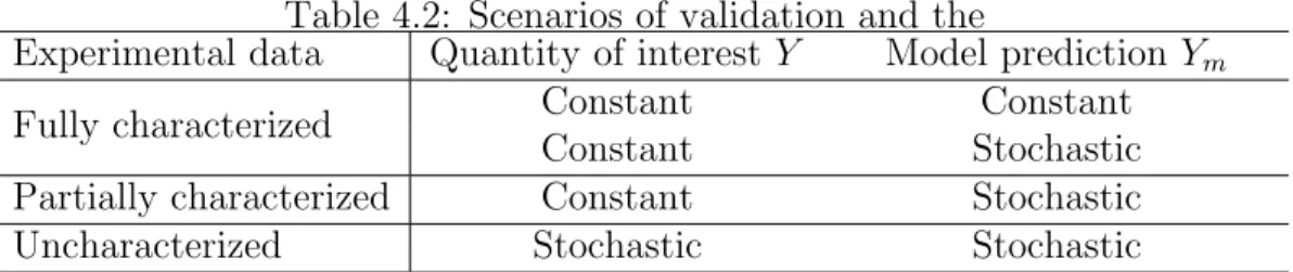
However, as discussed in Section 4.2, Y is actually a constant given a specific input x when the validation experiments are fully or partially characterized. Therefore, the reliability-based validation method can be used in cases where the validation attempts are fully/partially characterized.
Relationship between p-value, Bayes factor, and the reliability metric 75
- Relationship between p-value and the reliability metric
Similarly, the relationship between the Bayes factor and the p-value in the t-test can be obtained by combining Eq. 4.18, the relationship between the reliability-based metric r and the test statistic in the t-test or z-test is obtained as
Interpretation of quantitative model validation results
Reliability metric The threshold rth used in the reliability-based method represents the minimum probability that the difference d falls within an interval [−, ], and the decision to accept/reject a model can be made based on the decision maker's acceptable level of model reliability. Since the area metric has the physical unit for the quantity of interest and represents.
Detection of the directional bias
By comparing the values of r1 and r2 with the threshold rth/2 (half of the original threshold value because the width of intervals considered is half of the original one), the model can be judged to have failed the validation test if either r1 or r2 is less than rth/2. For example, if the model outputs at different test combinations are normal random variables, the values of Fxim(yDi) will all be less than 0.5 if yDi's are smaller than the mean of the corresponding normal variables.
Conclusion
It is noted that under certain conditions the p-value in a z-test or t-test can be mathematically related to the Bayes factor and reliability-based metrics. Bayesian model validation output and reliability-based metrics can be directly incorporated into long-term failure and device reliability analysis, explicitly accounting for model uncertainty [Sankararaman, 2012].
Introduction
In Section 5.4.1, the various quantitative model validation methods discussed in Chapter IV are used to validate a gas attenuation model. Furthermore, the error probability for the target unit is calculated based on the calibrated and validated models, as will be shown in Section 5.5.
Construction of a Bayesian network based on multi-scale and multi-
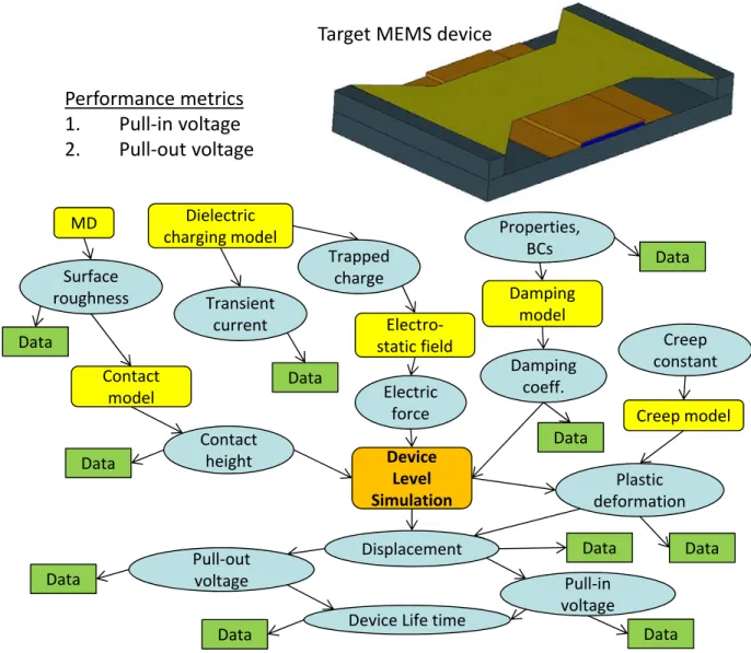
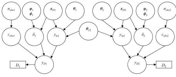
Both pull-in and pull-out voltage are important measurements when analyzing the reliability of a device after a certain period of use. Combining all the previously mentioned physical models, a schematic illustration of the entire BN is shown in Fig.
Bayesian network-based model calibration
- Calibration of dielectric charging parameters using a com-
- Calibration of multi-physics models using interval and point
- Different data on two devices
- Calibration with information flowing from left to
- Calibration with information flowing from right to
- Discussion
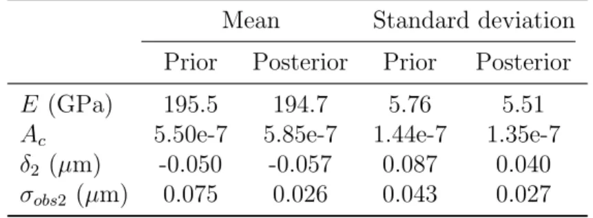
500,000 samples are collected and the fitted marginal posterior PDFs of the dielectric charge model parameters are shown in Fig. Then, the parameters in the right half of the Bayesian network are calibrated using the deflection data from Dev-2 and the posterior PDF of E obtained in the first step is used as .
Bayesian network-based model validation
- Validation of a damping model
- Modeling of micro-scale squeeze-film damping
- Experimental data for validation
- Classical hypothesis testing
- Bayesian hypothesis testing
- Reliability-based metric
- Area metric-based method
- Discussion
- Validation of calibrated dielectric charging model
- Validation of calibrated creep model
- Validation of device level simulation
It can also be observed that the failure rate of PCE model for pressure of 18798.45 Pa increases significantly in the test comparing r1 and r2 with rth/2 due to the existence of directional bias. The corresponding Bayes factors are shown in the subfigure titles of Fig.
Reliability of the target device
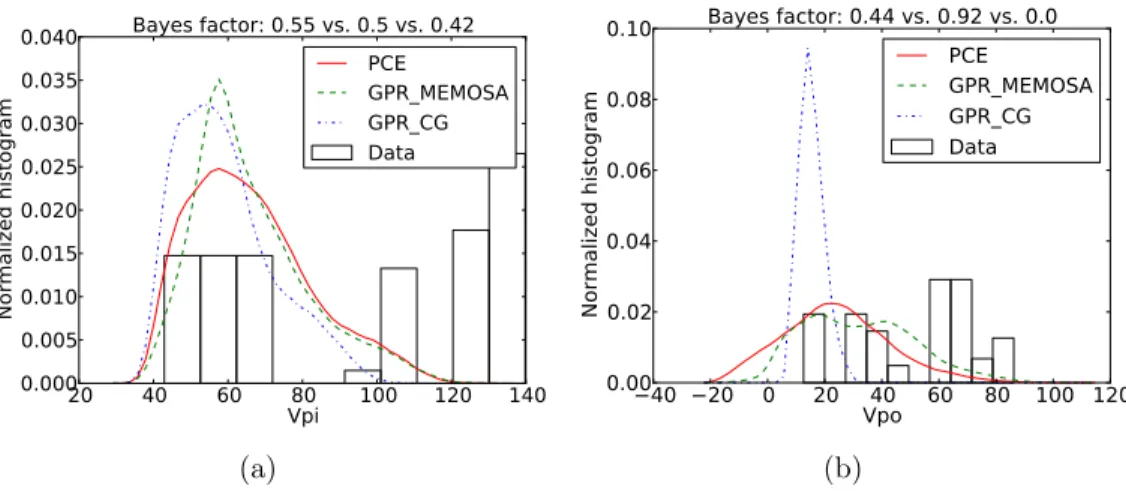
GPR CG" is chosen because the corresponding Bayes factor for the prediction of the tensile stress of the Die 10 D2 device is significantly higher than the other two surrogate models. Further, the surrogate models are constructed for changes in tensile and tensile stresses .
Conclusion
To account for the natural variation in loading and the uncertainty due to insufficient data, the coefficients of the ARIMA model are assumed to be random variables. The two subsets of data in Section 6.4.1 are also used to illustrate the Markov chain method and the update of the transition probability matrix.
INCLUSION OF TIME-DEPENDENT INPUT MONITORING DATA
Introduction
The autoregressive moving average (ARMA) method [Box et al., 1994] is based on time series analysis and characterizes the fatigue load spectrum in the time domain. It should be noted that all the three aforementioned methods are applicable for stationary load spectra, that is, the statistics of loading are assumed to be constant with respect to time.
Characterization of load history
- Rainflow counting method and stochastic reconstruction . 127
- ARIMA process loading
- Autoregressive integrated moving average (ARIMA)
- Identification of ARIMA model
- Uncertainty in the ARIMA model
- Direct updating of the characteristic matrix
- Bayesian updating of the ARIMA model
- Model Calibration based on the Bayes Theorem
- Continuous Bayesian updating of the ARIMA model 138
- Confidence assessment in load history prediction
The conditional probability density function f(Yt|Mi,ϕi,ωi,Y-t) of model output Yt of Mi for given values of ϕi and ωi can be constructed based on Eqs. A Bayesian updating approach is applied to the ARIMA model by calibrating the probability distributions of the model coefficients and the values of the probability weights.
Numerical example
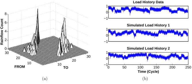
- Rainflow counting, stochastic reconstruction and updating 143
- ARIMA model method
- Partition of data set and initial model identification 146
- Confidence assessment of model prediction
According to the method presented in Section 6.2.2, the initial transition probability matrix is estimated using the first subset of data, and the simulated load spectrum samples are generated, as shown in Fig. The initial values of the weights are assumed to be equal to each other, meaning that two candidate models initially have the same probability of being the correct model for the loading history.
Conclusion
The use of the EIFS prior distribution before inspections is the same as in scenario 1. Some of the statistics, e.g., the model uncertainty statistics εcg, are assumed for the sake of illustration and can be conveniently substituted in practice if there more information available.
INCLUSION OF TIME-DEPENDENT SYSTEM HEALTH MONITORING
Introduction
Therefore, in addition to the extensive research efforts conducted separately at SHM and FDP, integration of these two technologies is desirable [Farrar and Lieven, 2007]. Two types of SHM data: real-time load monitoring data and ground crack inspection data are taken into account, and the uncertainty due to the monitoring technique is quantified in Section 7.2.
Crack inspection data
The dimensional accuracy is used to quantify the uncertainty in experimental crack growth data, with the following expression determined by regression analysis [Zhang and Mahadevan, 2001]. In practice, the accuracy of the size measurement can also be represented by other probabilistic models, depending on the actual experimental data of a specific NDI technique [Heasler et al., 1993].
Fatigue damage prognosis under uncertainty
- Fatigue crack growth simulation under multi-axial variable
- Uncertainty quantification in fatigue crack growth simulation162
- Connection of uncertainty sources using a Bayesian
- Probabilistic sensitivity analysis
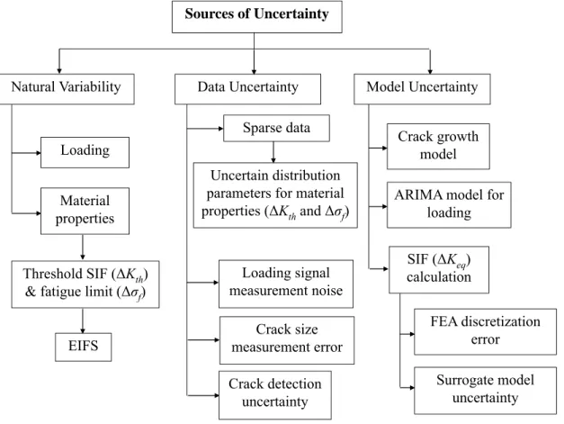
An investigation into various sources of uncertainty in fatigue crack growth simulation is presented in this section. In this chapter, all Xi's indicate the various sources of uncertainty in fatigue crack growth prediction as classified in Section 7.3.2.1.
Use of crack inspection data within prognosis
- Inference of EIFS using crack inspection data
- Strategy of prognosis for components in a fleet
- Validation of prognosis with new crack inspection data
7.3; π(am|aN) is the conditional probability density function of the measured crack size for a given actual crack size, which can be derived from Eq. The use of the previous EIFS distribution before inspection and the estimation of the current crack size based on the measured crack size is the same as in Scenario 1.
Numerical example
- Problem description
- Uncertainty and error quantification
- Usage of structural health monitoring data
- Characterization and prediction of loading sequence 177
- Prognosis for components in a fleet
- Validation of prognosis results
Note that some of the statistics in Table 7.2 can be found in the literature, such as the statistics of. The previous and updated PDFs of the coefficient ϕ1 of the ARIMA(2,1,0) model are shown in Fig.
Conclusion
As pointed out in Section 3.3, the limitations of this method include: (1) it uses a linear approximation of the model and may therefore fail to detect non-identifiability if the model is highly non-linear; (2) it can only detect local non-identifiability since the Taylor series expansion is constructed based on the derivatives at a single point; (3) it does not apply to statistical models; and (4) it does not cover practical non-identifiability due to data quality. We also showed that under some conditions the p-value in the z-test or t-test can be mathematically related to the Bayes factor and the reliability-based metric.
Overall reliability of model predictions
Three types of validation experiments and the corresponding input-output
Scenarios of validation and the
Overall reliability of model predictions
Prior and posterior statistics of parameters (with data on Dev-1)
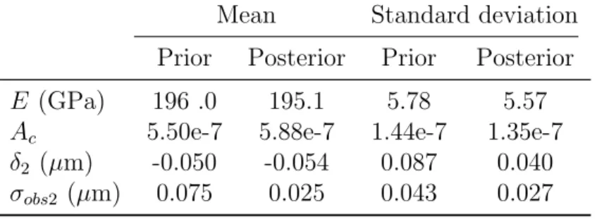
Prior and posterior statistics of parameters (with data on Dev-2)
Prior and posterior statistics of parameters (with data on Dev-2)
Prior and posterior statistics of parameters (with data on Dev-1)
Performance of PCE models in z-test with α = 0.05
Performance of PCE models in interval-based Bayesian hypothesis testing
Performance of PCE models in equality-based hypothesis testing with
Area metric for PCE models
Calculated Q statistics and the associated p-values
Overall predictive confidence for the three methods
Material and geometrical properties
Uncertainty quantification and associated statistics
Bayes factor and confidence assessment
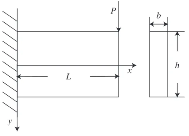
A thick cantilever subjected to point load at the free end
Actual model discrepancy versus least squares model discrepancy
Marginal posterior PDFs of Young’s modulus
Comparison between the predictions of calibrated beam model and calibra-
Comparison between the predictions of calibrated beam model and validation
Combined marginal PDF of Young’s modulus
Bayesian network for two physics models
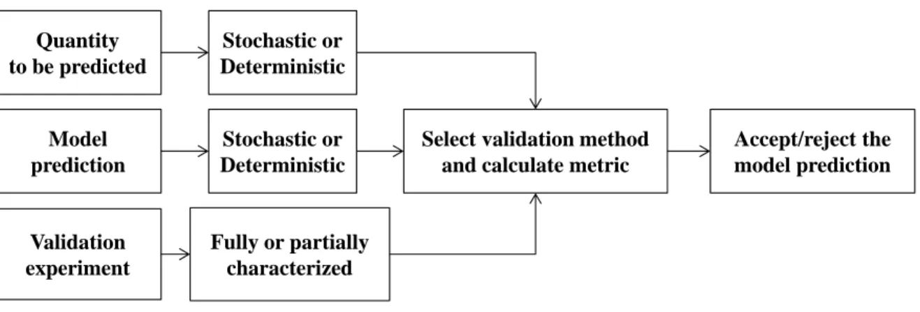
Decision process in quantitative model validation (Note: The last two steps
Graphical illustration of the combined test
Bayes network integration of various models and data for device-level
Marginal PDFs of dielectric charging model parameters
Comparison between the predictions of calibrated dielectric charging model
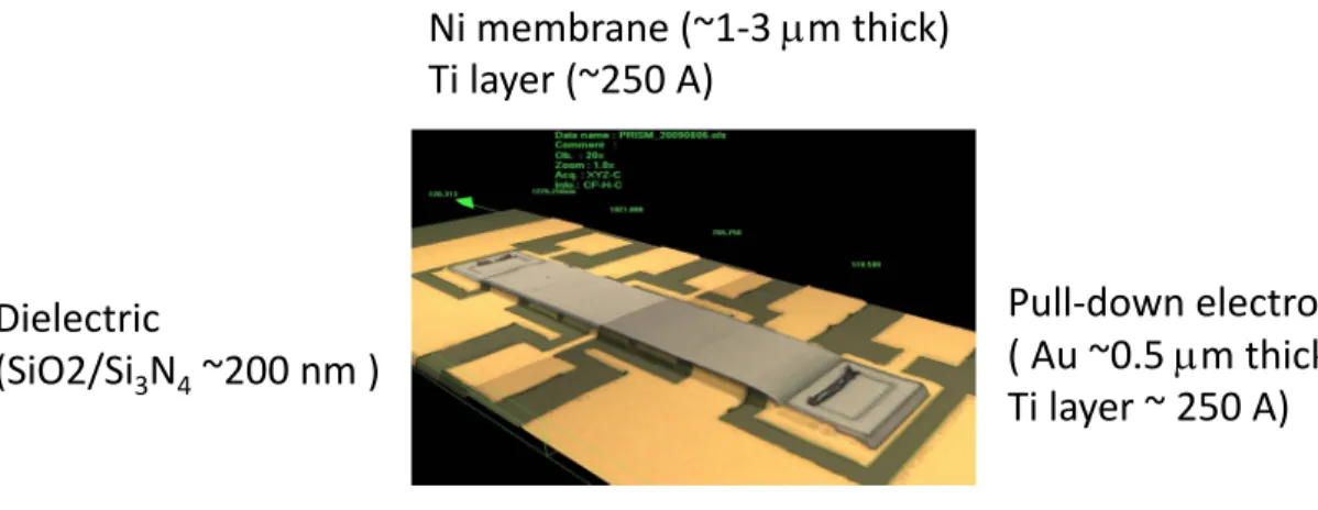
Example RF MEMS devices (Courtesy: Purdue PRISM center)
Bayesian network
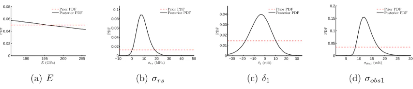
Calibration of parameters using pull-in voltage data
Calibration of parameters using deflection data
Calibration of parameters using deflection data
Calibration of parameters using pull-in voltage data
Example RF MEMS switch (Courtesy: Purdue PRISM center)
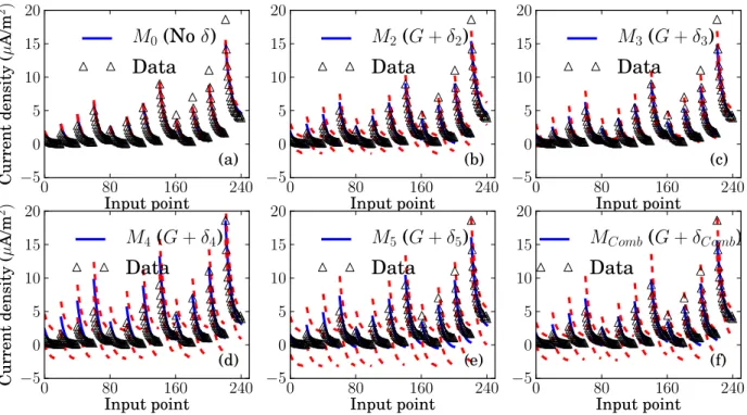
Graphical comparisons between PCE predictions and experimental data . 104
Bayes factor in interval-based hypothesis testing (on logarithmic scale)
Bayes factor in equality-based hypothesis testing (on logarithmic scale)
Reliability-based metric
Comparison of CDFs in the u-space and the physical space
Validation of the calibrated dielectric charging parameters using pull-out
Validation of the calibrated creep model using 25V data
Validation of the calibrated creep model using 45V data
Validation of the calibrated creep model using 58V data
Validation of the calibrated creep model using 30V data
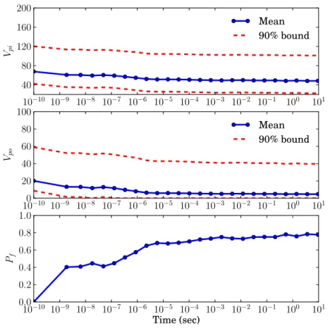
Inclusion of model uncertainty in pull-in and pull-out voltage prediction . 119
Probability of failure of the target device with the inclusion of model uncer-
A Scaled Helicopter Combat Maneuver Load History Data