If you have any comments about this topic guide, positive or negative, please use the form at the back of this guide. The University of London holds the copyright of all material in this handbook, except where otherwise noted.
This subject
Aims of the course
In this very short introduction, we aim to give you an idea of the nature of this topic and advise you on how best to approach it.
Learning outcomes
Second, we expect you to be able to "demonstrate knowledge and understanding" and you may be wondering how you will demonstrate this in the exam. Well, it is precisely by being able to successfully deal with invisible, non-routine questions that you will show that you understand the subject properly.
Route map to the guide
This is not something you should worry too much about: all maths subjects expect this and you will never be expected to do something that cannot be done with the material in that course.
Reading
Essential reading
Further reading
Online study resources
The VLE
Making use of the Online Library
Using the guide
Examination
This is not to cover every possible type of question that the examiners can think of. This way, you get used to facing unknown questions, struggling with them and finally finding a solution.
The use of calculators
You shouldn't let this detain you for too long: continue with the rest of the guide, and you'll pick up what you need as you go. There are many textbooks you can consult. For example, Chapter 2 of the Anthony and Biggs book may be helpful.
Some basic set theory
Sets
Subsets
Union and intersection
Showing two sets are equal
Numbers, algebra and equations
- Numbers
- Basic notations
- Simple algebra
- Powers
- Quadratic equations
- Polynomial equations
When n is a positive integer, then mag5 of the number a, denoted an, is simply the product of n copies of a, that is. Prove the power rules above using the definition of an for n∈N. The power a0 is defined as 1.
Mathematical statements and proof
Statement (d) is true exactly when one (or both) of the statements '21 is divisible by 3' and '21 is divisible by 5' are true. Statement (k) is an "if and only if" statement: it says that n2 is even for a natural number n exactly when n is even.
Introduction to proving statements
The most straightforward way to prove this is to assume that n is an even (that is, any) even number and then show that n2 is even. Another possible way to prove this result is to prove that if n2 is even, then n must be even.
Some basic logic
Negation
The negation of the universal statement 'for all n, p(n) is true' is the existential statement 'there is n such that ¬p(n) is true'. The negation of the existential statement 'there is n such that p(n) is true' is the universal statement 'for all n, ¬p(n) is true'.
Conjunction and disjunction
The negation of the universal statement 'for all n property p(n) holds' is the existential statement 'there is n such that property p(n) does not hold'. The denial (or refutation) of the statement “Every day it rains in London” is simple.
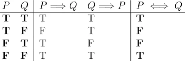
Implications, converse and contrapositive
Converse statements
In general, there is no reason why the opposite must be true just because the implication is. Activity 2.6 What is the opposite of the statement 'if the natural number n divides 4 then n divides 12'.
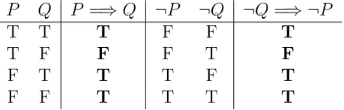
Contrapositive statements
Proof by contradiction
Some terminology
Alternatively, you can see that it is false because 2 is a counterexample: it is not divisible by 4, but it is divisible by 2. Let us prove by contradiction that there is no largest natural number. We then define what is meant by powers of a square matrix, look at its properties and how it interacts with the inverse of a matrix.
Definitions and terminology
We show how to algebraically manipulate matrices using these operations, and state what is meant by a zero matrix and an identity matrix. Then we define the transpose of a matrix and what is meant by a symmetric matrix, and look at the properties of the transpose of a matrix and how it interacts with the inverse of a matrix.
Matrix addition and scalar multiplication
Matrix multiplication
Matrix algebra
Matrices A and B must be of the same size, say m×n for the operation to be defined, so both A+B and B+A are also m×n matrices. Activity 3.8 If A is a 2×3 matrix, write the zero matrix for each of the rules involving addition.
Matrix inverses
Definition of a matrix inverse
To prove that the matrix B is equal to A−1, find the matrix products AB and BA and show that each product is equal to the identity matrix I. Activity 3.13 Verify that this is indeed the inverse of A by showing that if you multiply But on the left or right side of this matrix, then you get the identity matrix I.
Properties of the inverse
So if |A|=ad−bc6= 0, then to construct A−1 we take the matrix A, swap the main diagonal entries and put minus signs in front of the other two entries, then multiply by the scalar 1/ |A |.
Powers of a matrix
Transpose
The transpose of a matrix
This can be expressed as follows: The transposition of the product of two matrices is the product of the transpositions in the reverse order. It is important to understand why the product of the transposed values must be in reverse order by performing the following activity.
Symmetric matrices
The solutions to all exercises in the text can be found at the end of the textbook. This chapter of the topic guide closely follows the second half of Chapter 1 of the textbook.
Vectors in R n
Definition of vector and Euclidean space
Then we define the inner product of two vectors inRn and look at its properties. We then focus on developing geometric insight, starting with R2, looking at what we mean by the length and direction of a vector, and the angle between two vectors, and extending these concepts to R3.
The inner product of two vectors
This turns out to be particularly useful, and is known as the inner product or scalar product or dot product of v and w. It is important to realize that the inner product is just a number, a scalar, not another vector or a matrix.
Vectors and matrices
Developing geometric insight – R 2 and R 3
Vectors in R 2
We associate this point with the vector a= (a1, a2)T, as it represents the displacement from the origin (point (0,0)) to point A. For any other vector, v6=0, there is one unit vector in the same direction as v , namely.
Inner product
For example, we can use it to find the angle between two vectors by using cosθ = ha,bi. The nonzero vectors a and b are orthogonal (or perpendicular or sometimes normal) if the angle between them is θ = π2.
Vectors in R 3
Lines
Lines in R 2
Then the position vector of any point on the line is a sum of two displacements, which first go to the point (0,1) and then go along the line, in a direction parallel to the vector v= (1,2) T. As before, we can recover the Cartesian equation of the line by equating components of the vector and eliminating the parameter.
Lines in R 3
If you could move the crooked line in the floor up to the ceiling, the lines would intersect at a unique point. Two lines are said to be coplanar if they lie in the same plane, in which case they are either parallel or intersect.
Planes in R 3
To describe a plane that does not pass through the origin, we choose a normal vector n and a point P on the plane with position vector p. The orthogonality condition means that the position vector for any point on the plane is given by the equation.
Lines and hyperplanes in R n
Vectors and lines in R n
Hyperplanes
In this chapter we have defined and looked at vectors and Euclidean n-space, Rn, along with the definition and properties of the inner product in Rn. This chapter of the guide closely follows the first half of Chapter 2 of the textbook.
Systems of linear equations
We then learn an exact algorithm for using these operations to put the matrix into a form called reduced echelon form, from which the general solution of the system is easily obtained.
Row operations
So what are the operations we can perform on the equations of a linear system without changing the set of solutions? These operations do not change the set of solutions, since the constraints on the variables x1, x2,.
Gaussian elimination
- The algorithm — reduced row echelon form
- Consistent and inconsistent systems
- Linear systems with free variables
- Solution sets
Make sure you follow the algorithm to put the augmented matrix into reduced row form using row operations. In the abbreviated line of the echelon of this matrix, there are only three leaders.
Application: Leontief input-output analysis
After industries have used water and electricity to produce their output, how much water and electricity is left to satisfy outside demand. If, as before, we denote n×1 outside the demand vector by d, then in matrix form the problem we want to solve is to find the production vector x thus.
Homogeneous systems and null space
Homogeneous systems
The reduced row-echelon form of the augmented matrix of a system Ax=b will always contain the information for the solution of Ax=0, since the matrix A is the first part of (A|b). The solutions of the associated homogeneous system form an important part of the solution of the system Ax=b, which we will see in the next section.
Null space
The reduced row-degree form of the matrix A is the identity matrix (these are the first three columns of the augmented matrix). This is the reduced row degree form of the coefficient matrix, A. The reduced row degree form of any augmented matrix.
Elementary matrices
We examine the effects of a row operation on a matrix and on the product of two matrices. An elementary matrix, E, is an n×n matrix obtained by performing exactly one row operation on the then×n identity matrix, I.
Row equivalence
The main theorem
If the only solution of Ax=0 is x=0, then there are no free ones. non-leading) variables and the reduced row echelon form of A must have a leading in each column. Since each leading column has zeros elsewhere, this can only be the n×n identity matrix.
Using row operations to find the inverse matrix
We use the matrix A−1 to solve for x by multiplying the equation on the left by A−1,. If this is not possible (which will become apparent), the matrix is not invertible.
Verifying an inverse
Determine how to use the determinant to determine when a matrix A is invertible and to find the inverse matrix. We then prove the result that a matrix is invertible if and only if the determinant is nonzero, and see how to find the inverse of a matrix using cofactors and the adjoint matrix.
Determinants
This is a recursive definition, meaning that the determinant of an n×n matrix is given in terms of (n−1)×(n−1) determinants. Example 8.3 In the example we used (see page 117), instead of using the cofactor expansion along row 1 as shown above, we can choose to evaluate the determinant of the matrix A along row 3 or column 3, which will involve fewer calculations since is a33 = 0.
Results on determinants
Determinant using row operations
There is no change in the value of the determinant if a multiple of one series is added to another. The last steps all use RO3, so there is no change in the value of the determinant.
The determinant of a product
Matrix inverse using cofactors
The adjoint (called the adjugate in some textbooks) of the matrixA is the transpose of the matrix of cofactors. This consists of the cofactors from row 2 of A multiplied by the data from row 1, so it is equal to 0 according to Corollary 3 in section 8.2.
Cramer’s rule
Then, using Cramer's rule, we find x by evaluating the determinant of the matrix obtained from A by replacing column 1 with b,. We will complete the overview of the previous chapters with two new concepts, the rank of a matrix and the range of a matrix.
The rank of a matrix
Rank and systems of linear equations
The rank of the coefficient matrix A is 2, but the rank of the augmented matrix (A|b) is 3. Thus, the system Ax=b is consistent if and only if the rank of the augmented matrix is exactly the same as the rank of A.
General solution of a linear system in vector notation
Applying the same method in general to a consistent system of rank r with n unknowns, we can express the general solution of a consistent system Ax=b in the form This is a more precise form of the result of Theorem 6.2, which states that all solutions of a consistent system Ax=b are of the form x=p+z, where p is any solution of Ax=b and z∈N(A) , the null space of A (the set of all solutions of Ax=0).
Range
The system of equationsAx=b is consistent if and only if bis is a linear combination of the columns of A. You can use any solution x (so any value of s, t ∈R) to write b as a linear combination of the columns of A , so this can be done in an infinite number of ways.
Sequences
- Sequences in general
- Arithmetic progressions
- Geometric progressions
- Compound interest
- Frequent compounding
This process is known as compound interest (or compound interest), because interest is paid on interest previously added to the account. If the interest is added quarterly (so that 2% is added four times a year), the amount becomes after one year.
Series
Arithmetic series
Geometric series
Finding a formula for a sequence
Limiting behaviour
Financial applications
Use the formula for the sum of a geometric series to derive the formula for the value of an investment An after n years. St is the sum of the first terms of a geometric progression with the first term 2/3 and the total ratio 2/3, so.
First-order difference equations
Solving first-order difference equations
To see why this is true, first note that the difference equation can be written as yt−ayt−1 =b. R Read section 3.2 of Anthony and Biggs' book for a slightly different (and more complete) explanation of why this theorem is true.
Long-term behaviour of solutions
The cobweb model
Financial applications of first-order difference equations
First, we may want to know how large withdrawals can be made on an initial investment of P if we want to be able to withdraw I every year for N years.
Homogeneous second-order difference equations
The specific solution of the difference equation with these initial conditions is found by substituting t = 0 and d = 1 into the general solution. When the auxiliary equation has only one solution, α, the general solution is yt=Ctαt+Dαt= (Ct+D)αt.
Non-homogeneous second-order equations
Behaviour of solutions
Economic applications of second-order difference equations
Solve this equation and show that the price eventually adjusts to the clearing value (ie, the price at which supply and demand are equal) if and only if. Solution to Exercise 11.4 The auxiliary equation is. a) The differential equation can be derived in several ways.
Vector spaces
Definition of a vector space
A vector space, as we have defined it, is called a real vector space, to emphasize that the 'scalars' α, β and so on are real numbers and not (say) complex numbers. There is a notion of complex vector space, where scalars are complex numbers, which we will not cover.
Examples
Example 12.4 The set of m×n matrices with real entries is a vector space with the usual addition and scalar multiplication of matrices. The 'zero vector' in this vector space is the zero m×n matrix, which has all entries equal to 0.
Subspaces
An alternative characterisation of a subspace
We have seen that a subspace is a nonempty subset W of a vector space that is closed under addition and scalar multiplication, meaning that if u,v∈W and α∈R, then u+v and αvar are in W.
Subspaces connected with matrices
Null space
Range
To show that S1 is not a subspace, you need to find one counterexample, one or two specific vectors in S1 that do not satisfy the closure properties, such as.
Linear span
Lines and planes in R 3
Row space and column space
Linear independence
Testing for linear independence in R n
Basis
Coordinates
Dimension
Dimension and bases of subspaces
Finding a basis for a linear span in R n
Basis and dimension of range and null space
Linear transformations
Examples
Linear transformations and matrices
Rotation in R 2
Linear transformations of any vector spaces
Identity and zero linear transformations
Composition and combinations of linear transformations
Inverse linear transformations
Linear transformations determined by action on a basis
Range and null space
Rank and nullity
Coordinates and coordinate change
Change of basis and similarity
Matrices of linear transformations
Similarity
Eigenvalues and eigenvectors
Definitions
Finding eigenvalues and eigenvectors
Eigenspaces
Eigenvalues and the determinant
Diagonalisation of a square matrix
When is diagonalisation possible?
Powers of matrices
Systems of difference equations
Systems of difference equations
Solving by change of variable
Solving using matrix powers
Markov chains