Understanding Consumer Willingness to Pay: Methods and Applications in Marketing

37

implications

Kamel Jedidi and Sharan Jagpal*

Abstract

Accurately measuring consumers’ willingness to pay (WTP) is central to any pricing decision.

This chapter attempts to synthesize the theoretical and empirical literatures on WTP. We fi rst present the various conceptual defi nitions of WTP. Then, we evaluate the advantages and dis- advantages of alternative methods that have been proposed for measuring it. In this analysis, we distinguish between methods based on purchase data and those based on survey/experimental data (e.g. self-stated WTP, contingent valuation, conjoint analysis and experimental auc- tions). Finally, using numerical examples, we illustrate how managers can use WTP measures to make key strategic decisions involving bundling, nonlinear pricing and product line pricing.

1. Introduction

Knowledge of consumers’ reservation prices or willingness to pay (WTP) is central to any pricing decision.¹ A survey conducted by Anderson et al. (1993) showed that man- agers regard consumer WTP as ‘the cornerstone of marketing strategy’, particularly in the areas of product development, value audits and competitive strategy. Consider the following managerial questions you would face as a new product manager:

How does pricing a

● ffect the demand for my new product?

What price should I charge for my new product?

●

What is the likely demand for my new product if I charge this price?

●

What are the sources of demand for the new product? What fractions of this

●

demand come from cannibalization, switching from competitors, and market expansion? And which competitors will the new product affect most?

Which products in my product line should be bundled? And how much should I

●

charge for the bundle and for each of its components?

How should I determine my product mix and my product-line pricing policy?

●

If I can use a one-to-one marketing strategy, how should I customize prices across

●

consumers or consumer segments?

How should I determine the optimal quantity discount schedule for my product?

●

From the perspective of the standard economic theory of consumer choice, the key to answering all these questions is knowledge of consumers’ WTP for current and new product offerings in a category. Consider, for instance, a phone company that is planning to bundle its landline and wireless services. If the market researcher has information on

* The authors thank Vithala Rao, Eric Bradlow and Olivier Toubia for their comments.

1 Consistent with the literature, we shall use the term ‘willingness to pay’ interchangeably with

‘reservation price’. Alternative defi nitions will be discussed later in the chapter.

how much each of the target consumers is willing to pay for each of these services and the bundle, then it is straightforward to determine the optimal prices for the bundle and its components. As another example, suppose TiVo is planning to expand its digital video recorder (DVR) product line by offering a high-defi nition Series 3 DVR model. Suppose the market researcher knows how much each of the target consumers is willing to pay for this new product and each of the existing DVRs in TiVo’s product line. Suppose that s/

he also knows consumers’ WTP for generic boxes from cable companies. Then s/he can determine which consumers will switch away from the cable companies to purchase the new DVR (the customer switching effect), the extent to which TiVo’s new product will compete with the other DVRs in its own product line (the cannibalization effect), and how category sales are likely to expand (the market expansion effect) as a result of TiVo’s new offering. (See Jedidi and Zhang, 2002 for other examples.)

The practical importance of knowing consumers’ WTP is not limited to answering these managerial questions. Knowledge of WTP is also necessary for market researchers in implementing many other nonlinear and customized pricing policies such as bundling, quantity discounts, target promotions and one-to-one pricing (Shaffer and Zhang, 1995).

Furthermore, such knowledge bridges the gap between economic theory and marketing practice. Specifi cally, it enables researchers to study a number of other issues related to competitive interactions, policy evaluations, welfare economics and brand value.

There is a vast literature in marketing and economics on the measurement of WTP and its use for demand estimation, pricing decisions and policy evaluations (see Lusk and Hudson, 2004 for a review). In marketing, we are witnessing a renewed interest in the measurement of WTP (Chung and Rao, 2003; Jedidi et al., 2003; Jedidi and Zhang, 2002;

Wertenbroch and Skiera, 2002; Wang et al., 2007). This growing interest stems from three factors. First, pricing and transaction data (e.g. scanner panel data) are readily available to estimate consumer WTP. Second, the advent of e-commerce has made mass customiza- tion possible, thus motivating the need for more accurate measurement of WTP (Wang et al., 2007). Third, methodological advances in Bayesian statistics, fi nite mixture models and experimental economics allow one to obtain more accurate estimates of WTP at the individual or segment levels.

The goal of this chapter is to synthesize the WTP literature, focusing on the measure- ment of WTP and showing how this information can be used to improve decision-making.

The chapter is organized as follows. Section 2 presents the various conceptual defi nitions of WTP. Section 3 reviews the advantages and disadvantages of alternative methods that have been proposed to measure WTP. Section 4 illustrates how WTP measures can be used for various pricing decisions. Section 5 summarizes the main points and discusses future research directions.

2. Conceptual defi nitions of WTP

Jedidi and Zhang (2002, p. 1352) defi ne a consumer’s reservation price as ‘the price at which a consumer is indifferent between buying and not buying the product’. Formally, consider a consumer with income y, who is considering whether to buy one unit of product g priced at p or to keep her money. Let U(g, y 2 p) be her utility from buying the product and U(0, y) the utility from not buying it. Then, by defi nition, the consumer’s reservation price R(g) for product g is implicitly given by

U1g,y2R1g2 2 2U10,y2 ;0 (2.1) This is the standard defi nition of consumer reservation price in economics, and captures a consumer’s maximum WTP for product g, given consumption opportunities else- where and the budget constraint she faces. Jedidi and Zhang (2002) show that, under fairly general assumptions about the consumer’s utility function, the reservation price R(g) always exists, such that for any p # R(g) the consumer is better off purchasing the product. They also show that if the utility function is quasi-linear,² then faced with a choice among G products (g 5 1, . . ., G), to make the optimal choice decision a utility- maximizing consumer will need to know only her reservation prices for the product offer- ings and the corresponding prices for these products.

These theoretical properties imply that knowing a consumer’s reservation prices for the products in the category is sufficient to predict whether or not she will buy from the product category in question and which of these products she will choose. Specifi cally, the consumer will choose the product option that provides the maximum surplus (R(g) 2 p) subject to the constraint that p # R(g). She will not buy from the category if the maximum surplus across products is negative (i.e. for each product in the category, the consumer’s reservation price is always less than the price of that product). Thus knowledge of con- sumers’ reservation prices allows us to distinguish and capture three demand effects that a change in price or the introduction of a new product will generate in a market: the customer switching effect, the cannibalization effect and the market expansion effect.

Cannibalization (switching) results when consumers derive more surplus (R(g) 2 p) from a new product offering than from the company’s (competitors’) existing products. Market expansion results when non-category buyers now derive positive surplus from the new offering.

Other related defi nitions of WTP have been used in the literature. Kohli and Mahajan (1991) defi ne reservation price as the price at which the consumer’s utility (say for a new product) begins to exceed the utility of the most preferred item in the consumer’s evoked set (i.e. the set of brands which the consumer considers for purchase). That is, the reser- vation price for a new product is the price at which the consumer is indifferent between buying the new product and retaining the old one. Hauser and Urban (1986) defi ne reservation price as the minimum price at which a consumer will no longer purchase the product. Varian (1992) defi nes reservation price as the price at or below which a consumer will purchase one unit of the good. Ariely et al. (2003) argue for a more fl exible defi nition of reservation price. Specifi cally, they suggest that there is a threshold price up to which a consumer defi nitely buys the product, another threshold above which the consumer simply walks away, and a range of intermediate prices between these two thresholds in which consumer response is ambiguous.

Implicit in all these defi nitions of reservation price is a link to the probability of pur- chase (0 percent in Urban and Hauser’s defi nition, 50 percent in Jedidi and Zhang, and 100 percent in Varian’s). In order to reconcile these alternative defi nitions, Wang et al.

(2007) suggest that one should distinguish three reservation prices:

2 That is U1g,y2p2 5u1g2 1 a1y2p2 where u(g) is the utility of product g and a is a scaling constant.

(a) fl oor reservation price, the maximum price at or below which a consumer will defi - nitely buy one unit of the product (i.e. 100 percent purchase probability);

(b) indifference reservation price, the maximum price at which a consumer is indifferent between buying and not buying (i.e. 50 percent purchase probability); and

(c) ceiling reservation price, the minimum price at or above which a consumer will defi - nitely not buy the product (i.e. 0 percent purchase probability).

3. Methods to measure WTP

Reservation prices can be estimated from either purchase data or survey/experimental data. The following methods based on survey/experimental data are commonly used:

self-stated WTP, contingent valuation, conjoint analysis and experimental auctions. We consider several factors in evaluating the different measurement methods. The fi rst factor concerns incentive compatibility. That is, how accurate is the method in providing an incentive to consumers to reveal their true WTP? The second factor concerns hypotheti- cal bias. That is, how accurately can the method simulate the actual point-of-purchase context? Note that the issues of incentive compatibility and hypothetical bias are closely related to the conventional criteria of measurement reliability and internal and external validity in psychometric studies. The third factor pertains to the ability of the method to estimate reservation prices for new products with attributes that have not yet been made available in the market or have not varied sufficiently across products in the market to allow reliable estimation. A fourth factor relates to the ability of the method to measure WTP for multiple brands in a given category (e.g. different brands of toothpaste) or for multiple products across product categories (e.g. product bundles). This information is essential for estimating cross-price effects among new and competing products where the competing products could be products within a fi rm’s product line, product items in a bundle, or competitive products.

3.1 Methods based on actual purchase data

These methods analyze scanner/household panel data, test-market data, or simulated test-market data. They provide two important advantages. Because the input data come from actual purchases, these methods are incentive compatible and do not suffer from hypothetical bias. Household panel data, for example, provide useful information about consumers’ responses to the price changes of an existing brand and those of its competi- tors. Such information is useful for predicting the impact of a price change on category incidence, brand choice and quantity decisions (Jedidi et al., 1999). For new products, simulated test market methods such as ASSESSOR (Silk and Urban, 1978) and AC Nielsen BASES provide consumers with the opportunity to buy (real) new products at experimentally manipulated price points. In ASSESSOR, for example, participants are fi rst shown advertisements for the new and existing products. Then they are given seed money that they can keep or use to buy any of the available products displayed in a simulated store. This experimental design provides data on how the demand for the new product varies across the posted prices.

Despite these advantages, however, methods based on actual purchase data have several weaknesses. The main shortcoming is that, because of cost, the fi rm must choose a limited number of price points for its own product. In addition, the fi rm can examine only a limited number of price combinations for market prices across competitors. For

example, suppose Procter & Gamble (P&G) is competing against three brands in a par- ticular segment of the toothpaste market; in addition, P&G already has one brand of its own (say Crest) in that segment. Let’s say that P&G wishes to test the impact of two price points for a new brand that it plans to introduce in this market segment. For simplicity, assume that each of the four incumbent brands (including P&G’s own brand) can choose one of two price policies following the new product introduction. The fi rst is to continue with the current price and the second is to reduce price. Then, it will be necessary for P&G to run 32 (52⁵) separate experiments to examine all the feasible competitive scenarios before choosing a pricing plan for the new product.

In addition, as Wertenbroch and Skiera (2002) note, data from purchase experiments provide only limited information about WTP. To illustrate, suppose P&G conducts an ASSESSOR study for a new product. Let’s say that, for the posted set of prices for the new product and its competitors, 30 percent of the respondents purchase the new product. Then the only inferences that P&G can make are the following. Given the posted set of market prices, 30 percent of the respondents obtain maximum (positive) surplus by purchasing the new product. The remaining 70 percent of the respondents obtain maximum surpluses by buying another brand or not purchasing a brand in the product category. Note that this information is extremely limited. Specifi cally, since the experiment does not provide estimates of WTP per se, P&G cannot estimate new product demand for any other price for the new product or its competitors. Hence P&G cannot use the purchase data to determine the optimal price for the new product or the optimal product line policy.

3.2 Self-stated WTP

This method directly asks a consumer how much she is willing to pay for the product.

Consequently, this is perhaps the easiest method to implement. However, for a number of reasons, this method is likely to lead to inaccurate results. Perhaps the most serious problem is that the consumer is not required to purchase the product. Hence the meth- odology is not incentive compatible. A related problem is that consumers are likely to overstate their WTP for well-known or prestigious brands or for products they are keenly interested in. They are also likely to understate their WTP for less well-known brands or if they anticipate being charged a higher price for the product in the future. Finally, even if consumers are able to correctly state their WTP on average, this method will overstate the degree of heterogeneity in WTP in the population.³ Hence the fi rm will make suboptimal pricing decisions using self-stated WTP data.

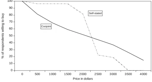
An interesting managerial question is whether self-stated WTP are similar to the esti- mates obtained by using other methods. Jedidi and Zhang (2002) examined the correla- tion between self-stated WTP for different brands of notebook computers and WTP that were estimated using a conjoint experiment. (We shall discuss the conjoint methodology in subsection 3.4.) The results for two brands showed that the correlations were low (0.43 and 0.28 respectively). The correlation coefficient for the third brand was not statistically signifi cant. Furthermore, the self-stated WTP led to excessively high estimates of demand

3 The variance of the observed WTP is always greater than or equal to the variance of the true WTP.

at low prices and signifi cantly understated the demand at high prices. Figure 2.1 shows the demand functions obtained from both methods for a Dell notebook computer with 266 mHz in speed, 64 MB in memory, and 4 GB in hard drive.⁴ These results strongly support the observation in the previous paragraph that the fi rm should not use self-stated WTP to make pricing decisions.

3.3 Contingent valuation methods

Contingent valuation (CV) is a popular WTP measurement method in agricultural eco- nomics and in determining the economic impact of changes in social policy. This method uses dichotomous choice questions to arrive at an estimate of WTP for each respondent in the experiment. In a marketing CV study, the researcher presents consumers with a new product, including its price, and asks them whether they would buy the new product at the listed price (Cameron and James, 1987). Thus a yes response indicates that the consumer is willing to pay at least the listed price for the new product. When these yes responses are aggregated across consumers, one obtains a demand curve that shows how the propor- tion of yes responses varies across the experimentally manipulated price levels.

Estimating WTP from CV data is straightforward using a binary choice model such as logit or probit (Cameron and James, 1987). In such a choice model, the decision of whether to buy or not is modeled through a latent utility function that depends on product characteristics and consumer background variables. Let p_i be the price of the new product given to consumer i. Let I_i be a variable that indicates whether consumer i decided to buy 1I_i512 or not 1I_i502. Let U_i5x^riâ 1 e_i be the latent utility of the

4 The percentage willing to buy is the percentage of respondents whose WTP is higher than the observed price.

Conjoint

Self-stated

0 10 20 30 40 50 60 70 80 90 100

0 500 1 000 1 500 2 000 2 500 3 000 3 500 4 000

Price in dollars

% of respondents willing to buy

Figure 2.1 Conjoint versus self-stated demand estimates

product concept, where x_i is a vector of explanatory variables that includes product char- acteristics (excluding price) and individual-specifi c consumer background variables, â is a vector of associated parameters, and Piis an error term. Then the binary choice model is given by

I_i5 e1 ifUi2pi.0

0 otherwise (2.2)

Since the price coefficient is set to 21 in equation (2.2), U_i2p_i is a measure of consumer surplus and U_i is therefore a direct measure of WTP. In this model, the â parameters capture the marginal WTP for each of the explanatory variables included in the model.

The main advantage of the CV method is that it is easy to implement. However, the method has several weaknesses. The CV method allows the researcher to observe only whether an individual’s WTP is higher or lower than the listed price. Hence it may be necessary to use large samples or multiple replications per respondent to obtain accurate results.

One modifi cation of the basic CV method is to use a sequential approach to obtain more precise information about WTP. In the fi rst step, the researcher asks a consumer to respond to a dichotomous (yes–no) question. Depending on the response, the researcher asks the consumer an additional dichotomous follow-up question. Specifi cally, if the initial response is no (yes), then the consumer is asked whether she would buy the new product at a lower (higher) price. This data collection procedure is called a double- bounded dichotomous choice question (Lusk and Hudson, 2004). Although this sequen- tial method can provide more information on the true WTP, it is subject to starting-point biases (i.e. the consumer’s response to the follow-up question depends on the initial price offered; see Shogren and Herriges, 1996; Hanemann et al., 1991).

Research evaluating the CV method suggests that it is not incentive-compatible and is also subject to hypothetical bias. For example, Bishop and Heberlein (1986) found that WTP in the hypothetical condition were signifi cantly overstated compared to those in the actual cash condition. Finally, in a meta-analysis of 14 valuation studies using the CV method, List and Gallet (2001) found that, on average, subjects overstated their WTP by a factor of 2.65 in hypothetical settings.⁵ However, the overstatement factor was much lower for private goods (51.65) compared to public goods (55). This fi nding is intuitive since most subjects are more confi dent in valuing products they commonly purchase than in valuing products that they may be unfamiliar with (e.g. public goods).

Most applications of the CV method vary list prices across consumers while holding the product concept description constant. In principle, the basic CV method can be modi- fi ed so that data on WTP for different combinations of price and product concepts (which are typically multidimensional) are obtained. However, as discussed earlier, the experi- mental design becomes very expensive and unwieldy. Thus the CV method is not feasible for predicting WTP when the fi rm is considering several alternative product designs – as is generally the case. Finally, and most importantly from a strategic viewpoint, the CV

5 The overstatement factor is calculated as the ratio of the mean hypothetical WTP to the mean actual WTP. The actual WTP are obtained from experiments with real economic commitments.

method considers only one product. Thus the fi rm cannot determine the separate effects of the new product (including product design and price) on brand switching, canni- balization and market expansion. Without this disaggregate information across different products and segments in the market, the fi rm cannot choose its optimal product-line policy. In particular, the fi rm cannot determine the net effect of its new product policy on product-line sales and profi ts after allowing for competitive reaction.

3.4 Conjoint analysis

Conjoint analysis is a popular WTP measurement method in marketing, transportation and environmental economics. Two common types of conjoint studies are the rating- based and the choice-based conjoint (CBC) methods. In a rating-based conjoint study, researchers present consumers with a number of hypothetical product profi les (concepts) and ask them to rate each of these profi les on a preference scale.⁶ Sometimes researchers ask consumers to proceed sequentially (Jedidi et al., 1996). In the fi rst step, consumers decide whether or not they will consider a particular product profi le for purchase. In the second step, consumers rate only those profi les that they are willing to consider (i.e.

profi les in the consideration set). In contrast, in a CBC study, researchers present con- sumers with several sets of hypothetical product profi les and ask them to choose at most one from each set.

To illustrate the conjoint methodology, consider the following example. Suppose a yogurt manufacturer is planning to introduce a new type of yogurt into the marketplace.

The fi rst, and perhaps most important, step is to determine the salient attributes. (See Lee and Bradlow, 2007 for an interesting approach for deriving attributes and levels using online customer reviews.) Let’s say that the fi rm has determined that the relevant attributes are the quantity of yogurt in a container, whether or not the yogurt is fat-free, the fl avor of the yogurt, the brand name (e.g. Dannon, Breyers, Yoplait) and the price.

Then a product profi le (or equivalently product concept) consists of a particular combi- nation of attributes including price. For example, one product profi le is the following: a 6-ounce, fat-free, vanilla-fl avored yogurt that is made by Yoplait and priced at $1. In a rating-based conjoint experiment, the researcher fi rst determines the set of profi les to be evaluated. Then consumers provide preference rating scores for all profi les that they are asked to evaluate. If a sequential approach is used, consumers fi rst sort profi les and then provide ratings scores for those profi les that they consider acceptable.

In a CBC experiment, the researcher fi rst determines the sets of profi les that consumers will be asked to evaluate. For example, one set of profi les might contain the following options: a 6-ounce, fat-free, vanilla-fl avored yogurt made by Yoplait and sold at a price of $1 (Alternative 1); a 10-ounce, full-fat, chocolate-fl avored yogurt made by Dannon and sold at a price of $1.50 (Alternative 2); and the no-purchase option (Alternative 3).

Then the consumer’s task is to choose one of these three alternatives. Similarly, the con- sumer is offered different sets of profi les and asked to pick the best alternative for each profi le in that set. A critical feature of the experimental design is that the no-purchase option must be included in each set of profi les that the consumer is asked to evaluate.

6 Our discussion of conjoint analysis is based on the full-profi le method. That is, the consumer is given information about all product attributes simultaneously.

This no-purchase alternative must be included so that we obtain unambiguous monetary values for the WTP. (See appendix in Jedidi et al., 2003.)

Whether the CBC or rating-based conjoint method is used, the product profi les or choice sets included in a study must be carefully chosen using an efficient experimental design (Louviere and Woodworth, 1983). Regardless of the method used for data collec- tion, the end result of a conjoint study is an estimated, individual-level utility function that describes how the consumer trades off different attributes.

The key question is the following: how can one use the conjoint results to infer consum- ers’ WTP for different product designs? Using basic principles from the economic theory of choice, Jedidi and Zhang (2002) show how to derive consumers’ reservation prices for a product from the individual-level estimates of conjoint coefficients. Let x_j be a vector that describes the attribute levels of product profi le j and â_i be the vector of the associ- ated parameters (part-worth coefficients) for consumer i.⁷ Let p_j be the price of profi le j and y_i be consumer i’s income.⁸ Then the (quasi-linear) utility consumer i derives from purchasing one unit of product j is U_ij5x^riâi1 a_i1yi2pj2, where a_i denotes the effect of an increase in income (the income effect) or of a decrease in price (the price effect). For any set of profi les in a choice set, if the consumer chooses the no-purchase option (i.e.

she decides to keep the money), then her utility is simply U_ij5 a_iy_i. Using the defi nition in equation (2.1), Jedidi and Zhang (2002) show that for this utility specifi cation, a con- sumer’s reservation price for product profi le j is defi ned by

R1j2 5x^rja^{^}i

a_i (2.3)

To illustrate the relationships among the conjoint part-worth coefficients and reserva- tion prices, suppose we conduct a CBC study and obtain the following individual-level utility function for consumer i for product j:

U_ij50.210.15 Dannon10.05 Yoplait10.15 Banana20.10 Strawberry20.5 Price where Breyers and Vanilla, respectively, are the base-level brand and fl avor and price is measured in dollars.⁹ Thus, for this consumer, the reservation price for the Yoplait brand that has a Banana fl avor is $0.80 5 (0.2 1 0.05 1 0.15)/0.5. In addition, a $1 change in price refl ects a utility difference of 0.5. Therefore every change of one unit in utility is equal to $2.00 in value (51/0.5). This ratio is what Jedidi and Zhang (2002) defi ne as the

‘exchange rate’ between utility and money for the consumer. In the example, the exchange rate implies that, for any product fl avor, consumer i is willing to pay up to an additional

$0.10 to acquire a Yoplait relative to a Breyers yogurt (50.05 3 $2.00).

Conjoint analysis, in its CBC form, can be viewed as an extension of the conventional

7 For simplicity, we assume that there are no interactions among the product attributes. The analysis can easily be extended to allow for such interactions in conjoint models.

8 The consumer’s income need not be observable, but one has to postulate its existence to develop an economic model.

9 In any conjoint experiment, it is necessary to choose a base level for each product attribute (e.g.

brand and fl avor in the yogurt example). The choice of base levels does not affect the results.

contingent valuation (CV) method in two ways. First, in CV, the product to be evalu- ated is typically fi xed across respondents. In contrast, the product profi les in conjoint experiments are experimentally manipulated, hence resulting in a within-subject design.

Second, conjoint analysis provides additional information about reservation prices. Thus CV provides information only about whether or not the new product is chosen. In con- trast, CBC provides detailed information about the case where the new product is not chosen. Specifi cally, one can distinguish whether the consumer who does not purchase the new product chooses another product (brand) alternative or the non-purchase option.

Because of this additional information, CBC provides several important advantages over CV. The choice task in CBC is more realistic than in CV and closely mimics the consumer’s shopping experience. Hence CBC minimizes hypothetical bias. Interestingly, previous research fi ndings show that the responses to CBC questions are generally similar to those from experiments based on revealed preference (e.g. Carlsson and Martinsson, 2001). In the few cases where the differences in the results from the two methodologies are statistically signifi cant, the differences are small (Lusk and Schroeder, 2004). An additional advantage of CBC is that, when the experiment manipulates several attributes simultaneously, consumers are more likely to consider other attributes than price in making the choice decision. Consequently, the task becomes more incentive-compatible.

From a managerial viewpoint, perhaps the most important advantage of CBC is the fol- lowing. In contrast to CV, CBC provides disaggregate information that allows the fi rm to distinguish how much of the demand for the new product comes from brand switching, cannibalization and market expansion. Consequently, the fi rm can choose the optimal product-line policy after allowing for the likely effects of competitive reaction following the new product introduction.

The estimation of conjoint models is straightforward regardless of whether we have choice or preference rating data.¹⁰ With rating-based data, one can use regression to esti- mate the conjoint model. In the special case where consumers provide rating scores only for profi les that are in their consideration sets, one can use a censored-regression model such as tobit to estimate the conjoint model (see Jedidi et al., 1996). With CBC data, the individual-level conjoint model is typically estimated using a hierarchical Bayesian, multinomial logit (MNL) or probit model (Jedidi et al., 2003; Allenby and Rossi, 1999).

The primary advantage of the MNL model is computational simplicity. However, the MNL method makes the restrictive assumption of independence of irrelevant alternatives (i.e. the ratio of the choice probabilities of two alternatives is constant regardless of what other alternatives are in a choice set). If researchers are interested in obtaining segment- level estimates of WTP, they can use fi nite-mixture versions of these models.

Although the methods described above will work in many cases, there are a number of potential pitfalls that one can encounter when estimating WTP. The quasi-linear utility model that we have discussed above is strictly linear in price. While this specifi cation is consistent with utility theory, a consumer’s reaction to price changes need not be linear,

10 Software for estimating conjoint models is readily available (e.g. SAS, SPSS and Sawtooth Software). Note that one does not need to observe consumer’s income to infer WTP. Because a_iyi

is specifi c to consumer i, it cancels out in a choice model and gets absorbed in the intercept in a regression model.

especially when the price differences across alternatives are large. In such cases, Jedidi and Zhang (2002, p. 1354) suggest using the exchange rate that corresponds to the price range that the fi rm is considering for the new product. Another issue arises if the price coefficient a_i is unconstrained and the estimated coefficient has the wrong sign for some consumers.

Thus, suppose some consumers use price as a signal for quality. In such a case, price has two opposing effects. On the one hand, it acts as a constraint since the higher the price paid, the worse off the consumer is. On the other hand, since price is a signal of quality, the higher the price, the higher the utility. Because of these competing effects, it is possible that the estimated WTP measures for these consumers will be negative; see equation (2.3).

Another potential difficulty can arise if the price coefficient for a particular respondent is extremely small (close to zero). This can happen if consumers are insensitive to price changes or the data are noisy. In this case, the exchange rate (and hence WTP) may be large and can even approach infi nity. One way to address these difficulties is to constrain the price coefficient so that lower prices always have higher utilities. Another frequently used approach is to constrain the price coefficient to be the same across consumers in the sample (e.g. Goett et al., 2000). A third approach is to constrain the price coefficient to 1 (see equation 2.2). In a choice model, this means that consumers maximize surplus instead of utility. The latter two methods are equivalent if the utility function is quasi-linear (see Jedidi and Zhang, 2002). In most practical applications, all three approaches lead to price coefficients that are non-zero and have the proper signs.

3.5 Experimental auctions

Auction-based methods are beginning to gain popularity in marketing because they measure real and not self-stated choices. We discuss below the following auction mecha- nisms: the Dutch auction; the fi rst-price, sealed-bid auction; the English auction; the nth- price, sealed-bid auction (Vickrey, 1961); the BDM method (Becker et al., 1964); and the reverse auction (see Spann et al., 2004).

In a Dutch auction, the opening price is high and is progressively lowered until one bidder is willing to purchase the item being auctioned. Thus the only information that is available to the fi rm is that the winner’s WTP is at least as high as the price at which the item was sold; in addition, the WTP of all other bidders are lower than this price.

Given this auction mechanism, a bidder’s bidding strategy will depend on her beliefs about others’ bidding strategies; in addition, her strategy will depend on her risk attitude.

Consequently, all bidders have an incentive to underbid. In particular, the person with the highest reservation price may not always submit the highest bid. Note that, from a mana- gerial viewpoint, the information from a Dutch auction is extremely limited. All that the fi rm knows is the (potentially understated) maximum price at which it can sell one unit of its product. Thus, suppose there are three bidders (A, B and C) and A wins the auction at a bid price of $200. Then the only quantitative demand information available to the fi rm is the following. If it sells one unit, it can obtain a minimum price of $200. However, since bidders have an incentive to underbid, this price may be too low. Furthermore, the results provide no information about market demand if the fi rm plans to sell more than one unit in the marketplace.

In the fi rst-price, sealed-bid auction, each bidder submits one bid. This information is submitted to the auctioneer and is not provided to the other bidders. The highest bidder wins the auction and pays her bid price. Note that, as in the Dutch auction, each bidder

has an incentive to bid less than her reservation price. However, in contrast to the Dutch auction, the fi rm obtains more detailed information about the demand structure for its product. Thus, suppose there are three bidders (A, B and C) as before. Let’s say that the sealed bids are as follows: A bids $100, B bids $160, and C bids $250. Then the fi rm knows the following information about demand. If it wants to sell one unit, the minimum price that it can charge is $250 per unit. If it wants to sell two units, the minimum price that it can charge is $160 per unit. If it wants to sell three units, the minimum price that it can charge is $100. Note that, in contrast to the Dutch auction, the fi rm obtains market demand information for different volumes. However, since all bidders have an incentive to underbid, the fi rm is likely to choose a suboptimal price.

In an English auction, participants offer ascending bids for a product until only one participant is left in the auction. This bidder wins the auction and must purchase the auctioned product at the last offered bid price. Note that, in contrast to the fi rst-price, sealed-bid auction, the English auction is an ‘open’ auction. Specifi cally, all bidders know each other’s bids. This experimental design is useful in situations where it is important to incorporate market information into participants’ valuations (e.g. potential buyers are likely to communicate with each other). However, this method can be a limitation if consumers make independent valuations in real life (Lusk, 2003). In addition, because the bids are ‘open’, the last bid tends to be only marginally higher than the second-highest bidder’s last bid.

Note that, in contrast to the Dutch auction and the fi rst-price, sealed-bid auction, bidders in an English auction have an incentive to reveal their true reservation prices.¹¹ That is, a bidder will drop out of the auction only when the last bid exceeds her reserva- tion price. From a managerial viewpoint, the fi rm obtains much more detailed informa- tion about the market demand for its product. For simplicity, assume that there are three bidders (A, B and C). Suppose A drops out when the price is $10, B drops out when the price is increased to $15, and C purchases the product at a price of $16. These results imply the following market demand structure. If the fi rm wants to sell three units, the maximum price it can charge is $10 per unit. If the fi rm wants to sell two units, the maximum price it can charge is $15 per unit. Note that these results do not imply that the maximum price that the fi rm can charge for one unit is $16. Specifi cally, bidder C needs only to bid marginally more ($16) than bidder B, who drops out when the price is raised to $15. The only inference is that bidder C’s minimum reservation price is $16. From a practical viewpoint, it is likely that, in most cases, the fi rm will sell more than one unit.

Hence the fi rm can use the results of an English auction to determine what price to charge for its product.¹²

In an nth-price, sealed-bid auction (Vickrey, 1961), each bidder submits one sealed bid to the seller. None of the other bidders is given this information. Once bids have been made, the (n 2 1) highest bidders purchase one unit each of the product and pay an amount equal to the nth-highest bid. Perhaps the most commonly used nth-price auction

11 This conclusion of incentive compatibility holds if the auction is not conducted repeatedly with the same group of bidders and bidders cannot purchase more than one unit. If either of these assumptions does not hold, bidders may behave strategically and systematically choose bid prices that are lower than their WTP.

12 This analysis assumes that consumers will not purchase multiple items of the product.

is the second-price (n 5 2) auction in which the highest bidder purchases the product at the second-highest bid amount. Similarly, suppose the fi rm uses the fourth-price auction (n 5 4). Then the three highest bidders will purchase one unit each at the price bid by the fourth-highest bidder. Because of the sealed-bid mechanism, the participants in this auction learn only the market price and whether or not they are buyers in the auction.

As Vickrey (1961) shows, the second-price, sealed-bid auction is isomorphic to the English auction. This is because the fi nal price paid in both auctions is determined by the bid of the second-highest bidder. Furthermore, both the English and nth-price auction mechanisms are incentive compatible. Hence, in principle, the fi rm can use either the English auction or the nth-price, sealed-bid Vickrey auction to determine the optimal price when it sells more than one unit.¹³

Despite the theoretical advantages of the Vickrey auction methodology, the method has several drawbacks as a marketing research tool for measuring WTP (Wertenbroch and Skiera, 2002). The fi rst limitation concerns the operational difficulties in implement- ing the method in market research. The second stems from the fact that the bidding process in the auction does not mimic the consumer purchase process (Hoffman et al., 1993). The third limitation stems from the limited stock of products being auctioned. This is not only unrealistic for many products in retail settings; it also encourages participants to bid more than the true worth of the product to ensure that they are placing the winning bid (e.g. Kagel, 1995). Finally, empirical fi ndings suggest that low-valuation participants become quickly disengaged in these auctions when they are conducted in multiple rounds (Lusk, 2003). Thus subjects quickly learn that they will not win the auction and drop out of the auction by bidding zero.

To address some of these limitations, Wertenbroch and Skiera (2002) propose the use of the incentive-compatible, BDM (Becker et al., 1964) method for eliciting WTP. The BDM method is as follows. Each participant submits a sealed bid for one unit of the product. The auctioneer then randomly draws a ‘market’ price. If the participant’s bid exceeds this value, the participant is required to purchase one unit of the product at the market price. If the bid is lower than the market price, the bidder does not purchase the product. Note that, although the BDM method is structurally similar to the standard auction method, there is a fundamental difference. The BDM procedure is not an auction because participants do not bid against one another (Lusk, 2003).

One important practical advantage of the BDM procedure over standard auctions is that it does not require the presence of a group of consumers in a lab for bidding. This feature makes it possible to more accurately mimic the purchase decision process by elicit- ing WTP at the point-of-purchase (Wertenbroch and Skiera, 2002; Lusk et al., 2001). In addition, because the supply of the product is not limited, every consumer can buy the product as long as his or her WTP is greater than the randomly drawn price. This aspect makes low-valuation participants more likely to be engaged in the experiment. One draw- back of the BDM method is the absence of an active market such that participants can incorporate market feedback. Empirical fi ndings, however, suggest that the BDM method and the English auction generate similar results (Lusk et al., 2002; Rutström, 1998).

13 This result holds provided the auction is not repeated with the same group of bidders. For this scenario, bidders may behave strategically and not reveal their true reservation prices.

Another type of auction mechanism is the reverse auction – a method used by such Internet fi rms as Priceline.com. The reverse auction method works as follows. The seller specifi es a time period (e.g. the next seven days from now) during which it will accept bids to purchase a product. During this period, each bidder is allowed to submit one bid for the product.¹⁴ Only the seller has access to bids. The outcome of the auction is as follows. The seller has a secret threshold price below which she will not sell the product.

If a consumer bids more than the threshold price, the consumer must purchase one unit of the product at his or her bid price. If the consumer bids less than the seller’s threshold price, the seller will not sell the product to the consumer. Note that the reverse auction is similar to the BDM method in that bidders do not compete with each other. However, there is an important difference. In a BDM auction, the buyer pays the randomly drawn market price. In a reverse auction, each buyer pays her bid price if offered the option to purchase.

To illustrate how the reverse auction works, suppose a hotel wishes to sell excess cap acity (e.g. three room nights on a given Saturday one month after the auction is conducted).

Since the marginal cost of a room night is low, let’s say that the hotel’s secret threshold price per room night is $20. Suppose the fi rm conducts the reverse auction over a seven- day period and the room-night bids in descending order are as follows: $60 (Consumer A);

$50 (Consumer B); $40 (Consumer C); $30 (Consumer D); and a number of bids less than

$30. Then the hotel will choose the following room-night pricing plan. It will charge A a price of $60, B a price of $50, and C a price of $40 for the Saturday night stay. Note that, in contrast to standard auctions, consumers pay different prices for the same product. In our example, the reverse auction method allows the hotel to ration out the limited supply of room nights by using a price discrimination (price-skimming) strategy.

From a managerial viewpoint, reverse auctions are a mixed blessing. On one hand, they allow the fi rm to extract consumer surplus from the market by charging differential prices. Furthermore, they are a convenient, low-cost method for the fi rm to sell excess capacity without disrupting the price structure in traditional distribution channels. On the other hand, reverse auctions are not incentive compatible. Specifi cally, customers will bid less than their true WTP in order to obtain a surplus from the transaction. This lack of incentive compatibility reduces the ability of the fi rm to extract consumer surplus from the market. To address this problem, some researchers have suggested the follow- ing modifi cation: allow bidders to submit multiple bids but require each bidder to pay a bidding fee for each bid submitted (Spann et al., 2004).

3.6 Comparison of WTP methods

Experimental auctions (EAs) can provide several advantages over stated preference methods. Many auction methods are incentive compatible. That is, bidders have an incentive to reveal their true WTP. In contrast to stated preference methods, EAs are conducted in a real context that involves real products and real money. In addition, by putting subjects in an active marketing environment, some EAs allow one to estimate WTP after allowing for a market environment with feedback among buyers. Depending on the purchase context, this feature may be important. WTP from EAs are empirically

14 Some reverse auctions allow bidders to make multiple bids. See, e.g., Spann et al. (2004).

observed. Hence one can obtain individual-level estimates of WTP without making para- metric assumptions (e.g. normality) about the distribution of WTP in the population.

However, in spite of these advantages, the EA methodology is not a panacea for meas- uring WTP. The elicitation process does not mimic the actual purchase process that a consumer goes through, including search for information. The EA method focuses on one product/product design only. Hence one cannot measure the cannibalization, substitu- tion and market-expansion effects of a new product entry. Nor can one determine how consumers trade off attributes. Consequently, the EA method can be used only at a late stage of the product development process when the fi rm has fi nalized the product design and the remaining issue is to choose the price conditional on this product design. Since participants in an EA study are expected to pay for the products they purchase, the EA method cannot be used to determine the reservation prices for durables (Wertenbroch and Skiera, 2002). The EA method assumes that reservation prices are deterministic. This may not be the case, especially for new products or products with which the consumer is unfamiliar. It may be difficult to generalize the WTP estimates from an EA study to a national level because it is infeasible to recruit a sufficiently large and representative sample. Subjects must be recruited and paid participatory fees to attend laboratory ses- sions. This potentially introduces bias into the resulting bids (Rutström, 1998). Depending on the EA method used, bidder values may become affiliated (i.e. a relatively high bid by one auctioneer induces high bids from others). This degrades the incentive compatibility of an auction (Lusk, 2003). In addition, it is not uncommon to observe a large frequency of zero-bidding, potentially because of lack of participant interest (Lusk, 2003). Hence the fi rm obtains incomplete information about the demand structure in the market.

Empirical studies comparing WTP measures across methods are limited. In three studies, Wertenbroch and Skiera (2002) fi nd that WTP estimates from BDM are lower than those obtained from open-ended and double-bounded contingent valuation methods.

Similarly, Balistreri et al. (2001) fi nd that bids from an English auction are signifi cantly lower than those obtained from open-ended and dichotomous CV methods. Lusk and Schroeder (2006) fi nd that the WTP estimates from various auction mechanisms are lower than those from CBC. These fi ndings may be due to the incentive compatibility of the auction methods and to the hypothetical bias inherent in the CV and conjoint analysis methods. In contrast, Frykblom and Shogren (2000) found that they could not reject the null hypothesis that WTP estimates obtained from a non-hypothetical (dichotomous) CV method are equal to those obtained from a second-price auction.

3.7 Emerging approaches

A new stream of research is emerging in marketing that combines the advantages of the stated preference methods with the incentive compatibility of the BDM method. Ding et al. (2005) extended the self-stated WTP and CBC methods using incentive structures that require participants to ‘live with’ the consequences of their decisions. Using Chinese dinner specials as the context, the authors conducted a fi eld experiment in a Chinese restaurant during dinner time. For the self-stated condition, consumers were presented with a menu of 12 Chinese dinner specials (with no price information) and were asked to state their WTP for each meal in the menu. Consumers were told upfront that a random procedure would be used to select a meal from the menu and that they would receive this meal if their WTP exceeded a randomly drawn price. For the CBC condition, the authors

presented consumers with 12 choice sets of three Chinese meals each (with price informa- tion) and asked them to choose at most one meal from each choice set. Consumers in this condition were told upfront that a random lottery would be used to draw one choice set and that they would receive the meal that they selected from that choice set. (The con- sumer would receive no meal if she selected none of the meals in the choice set.) For both experimental conditions, the price of the meal (random price for the self-stated method and menu price for CBC) would be deducted from their compensation for participating in the study. The out-of-sample predictions show that the incentive-aligned conjoint method outperformed both the standard CBC and incentive-aligned, self-stated WTP methods.

More recently, Park et al. (2007) proposed a sequential, incentive-compatible, conjoint procedure for eliciting consumer WTP for attribute upgrades. This method fi rst endows a consumer with a basic product profi le and a budget for upgrades. In the next step, the consumer is given the option of upgrading, one attribute at a time, to a preferred product confi guration. During this process, the consumer is required to state her WTP for each potential upgrade she is interested in. In addition, the BDM procedure is used to ensure that the incentive-compatibility condition is met. That is, the consumer receives the upgrade only if her self-stated WTP for the upgrade exceeds a randomly drawn price for that upgrade. When no further upgrade is desired by the consumer or the con- sumer’s upgrade budget is exhausted, the consumer receives the fi nal upgraded product.

The authors tested their model using data collected from an experiment on the Web to measure consumers’ WTP for upgrades to digital cameras. The out-of-sample validation analysis shows that the new method predicted choice better than the benchmark (self- explicated) conjoint approach.

4. Using WTP for pricing decisions

So far, we have focused on empirical methods for measuring WTP. In this section we discuss how managers can use WTP measures to choose pricing policies. We discuss three application areas: bundling, quantity discounts and product line pricing decisions.

4.1 Bundling

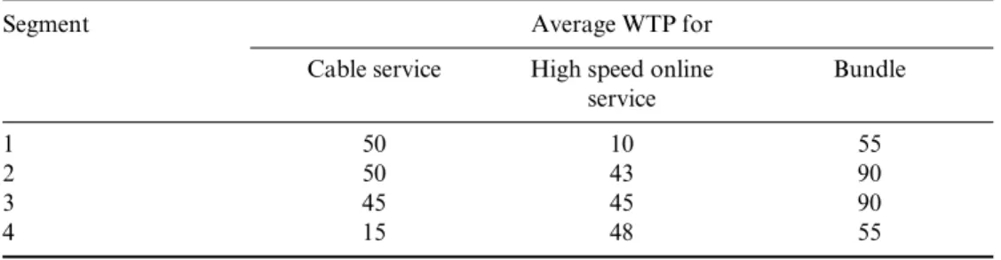
Consider a cable company, say Comcast, which sells two services: a basic digital cable service and high-speed online service. Suppose Comcast has conducted market research and obtained the WTP measures shown in Table 2.1 for its bundled and unbundled services for four segments in the market. (We shall discuss empirical methods to estimate the WTP for bundles later in this section.)

Table 2.1 WTP for individual services and bundle in dollars

Segment Average WTP for

Cable service High speed online service

Bundle

1 50 10 55

2 50 43 90

3 45 45 90

4 15 48 55

Suppose all segments are of equal size (1 million customers each) and the marginal cost of providing each service is zero. Then a consumer will only consider buying a particular service or bundle if the price charged is less than her WTP for that service or bundle.

In addition, she will choose the alternative that maximizes her surplus (5 WTP for any service or bundle – price of that service or bundle). If the maximum surplus is negative, the consumer will not purchase any of the services or the bundle.

Given this information about WTP and costs, Comcast can choose from among three pricing strategies: a uniform pricing strategy, a pure bundling strategy, or a mixed bun- dling pricing strategy. If Comcast uses uniform pricing, it will sell each service separately at a fi xed price per unit. If Comcast uses pure bundling, it will only sell the two services as a package for a fi xed price per package. If Comcast uses mixed bundling, it will sell the services separately and as a package.

Suppose Comcast uses a uniform pricing strategy. Then, using the WTP information in Table 2.1, we see that the optimal price for the cable service is $45. If this price is chosen, Comcast’s profi t from the cable service will be $135 million. Similarly, the optimal price for high-speed online service is $43 and the profi t from this service is $129 million. Hence Comcast’s product line profi t if it uses a uniform pricing strategy is $264 million (5 profi t from cable service 1 profi t from high-speed online service).

Suppose Comcast uses a pure bundling policy. Then the optimal price for the bundle is $55 and the product line profi t is $220 million. Finally, if Comcast uses a mixed bun- dling strategy, the optimal policy is to charge $90 for the bundle, $50 for the cable service alone, and $48 for the high-speed online service.Hence Comcast’s product line profi t will be $278 million (5 180 1 50 1 48). Consequently, the optimal product line policy is to use a mixed bundling strategy.

The previous discussion assumed that the manager knows the WTP for the individual products and the bundles. So far, we have discussed only how to estimate WTP for indi- vidual products. How can one estimate the WTP for product bundles? One way is to use self-stated WTP. However, as discussed, these are likely to be inaccurate, especially for new products or for products with which the consumer is unfamiliar. Another approach is to use the individual-level, choice-based method developed by Jedidi et al. (2003) or a modifi ed version that allows segment-level estimation. This method is philosophically similar to the choice-based methods discussed earlier. That is, consumers seek to maxi- mize their surpluses. As shown by Jedidi et al., their choice-based method provides more accurate estimates of reservation prices than the self-stated methodology. In practical applications, the data will be more complex than in the example above. For example, there will be many more segments, products and bundles. In such cases, the choice of the optimal bundling policy is complicated. One approach is to use an optimization algo- rithm (e.g. Hanson and Martin, 1990) to analyze the WTP results and cost data for the products and bundles in question.

4.2 Quantity discounts/nonlinear pricing

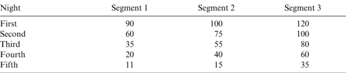
Suppose the Marriott Hotel seeks to determine how to price different packages for its standard rooms. Suppose the average WTP measures for stays of different durations in the hotel for three leisure segments are as shown in Table 2.2. Furthermore, assume that Marriott has sufficient room capacity to meet all demand.

Note that for any given consumer segment, the WTP is the highest for the fi rst night

and decreases for every successive night. Suppose the three segments are of equal size (1000 customers) and that the hotel’s marginal cost per room is approximately zero. (This is a reasonable assumption since most costs for maintaining hotel rooms are fi xed.) Hence any pricing policy that maximizes sales revenue also maximizes profi ts.

One option for Marriott is to set a uniform price per night, regardless of the duration of stay. Following the same procedure as in the bundling case, we fi nd that the sales- revenue maximizing price is $55 per night. If Marriott uses this uniform pricing plan, it will sell 9000 hotel night stays and obtain a revenue (gross profi t) of $495,000. An alterna- tive pricing strategy is to use a quantity discount pricing plan based on the ‘price-point’

method (see Dolan and Simon, 1996, p. 173). Using this approach, Marriott will proceed sequentially and set the revenue-maximizing price for each successive night stay. Table 2.3 presents the optimal pricing results using the price-point method.

Thus, for the fi rst night the optimal price is $90. This pricing policy leads to 3000 night stays and a revenue of $270,000. Conditional on this pricing policy, the optimal price for the second night is $60, yielding 3000 night stays and a revenue of $180,000. Conditional on the prices for the fi rst two nights, the optimal price for the third night is $55. Note that Segment 1 will not stay for a third night because its WTP for the third night ($35) is lower than the price for the third night ($55). Hence the hotel will sell 2000 night stays and obtain a revenue of $110,000. Similarly, we can determine the number of night stays and the corresponding revenues for the fourth and fi fth nights (see Table 2.3). Given this price-point strategy, Marriott will sell 11,000 night stays and make a gross profi t of

$675,000. Note that, when Marriott uses a quantity discount pricing plan, it sells more hotel room nights and obtains a higher profi t than if it uses uniform pricing. Specifi cally, the number of hotel night stays increases from 9000 to 11,000 (a 22 percent increase) Table 2.2 WTP in dollars for a hotel night for different stay durations

Night Segment 1 Segment 2 Segment 3

First 90 100 120

Second 60 75 100

Third 35 55 80

Fourth 20 40 60

Fifth 11 15 35

Table 2.3 Pricing of hotel night stays

Night Optimal price for nth

night ($)

Number of night stays Sales revenues ($)

First 90 3000 270,000

Second 60 3000 180,000

Third 55 2000 110,000

Fourth 40 2000 80,000

Fifth 35 1000 35,000

Total 11,000 $675,000

and gross profi ts increase even more sharply from $495,000 to $675,000 (a 36 percent increase).

As discussed, WTP information of the type presented in Table 2.2 can be collected in a number of different ways. For example, one can use conjoint or choice-based experiments where the quantity of product (e.g. different package sizes for a frequently purchased product or the number of hotel nights in the current example) is a treatment variable. See Iyengar et al. (2007) for an example of nonlinear pricing involving the sale of cellphone service. Alternatively, one can use different auction methodologies including the reverse auction method to estimate WTP.¹⁵

4.3 Product line pricing

In this section, we show how the fi rm can use information about WTP to determine its optimal product mix and product line pricing strategy after allowing for competition.

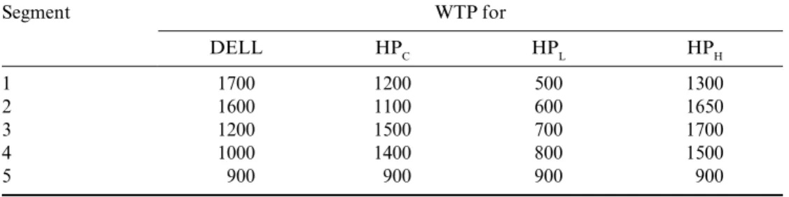
Consider the following hypothetical example from the PC industry. For simplicity, suppose there are two players in the PC notebook market: Dell and Hewlett-Packard (HP). Let’s say that in the fi rst period Dell sells one model of notebook (DELL) and Hewlett-Packard also sells one model (HP_C). Furthermore, there are fi ve segments, each of equal size (1 million), whose WTP for the DELL and HP_C notebooks are as shown in Table 2.4, columns 2 and 3, respectively.

Suppose the marginal costs for the DELL and HP_C notebooks are equal ($800 per unit). In addition, Dell and HP set the prices of their models simultaneously in the fi rst period. Consider the following pricing scenario. Let’s say that Dell charges a price of

$1200 for the DELL notebook and HP charges a price of $1400 for the HP_C model.

Then each consumer will choose the notebook model that maximizes her surplus. If the maximum surplus is negative, the consumer will not purchase either model. Given this set of prices, Segments 1 and 2 will purchase the DELL, Segments 3 and 4 will

15 Internet retailers (e.g. Priceline.com) often sell hotel room nights using the reverse auction methodology. Consequently, bidding information by consumers can be used to infer their WTP for purchasing different quantities of a product.

Table 2.4 WTP for different models of notebook computers by Dell and Hewlett- Packard ($)

Segment WTP for

DELL HP_C HP_L HP_H

1 1700 1200 500 1300

2 1600 1100 600 1650

3 1200 1500 700 1700

4 1000 1400 800 1500

5 900 900 900 900

Note: DELL 5 The notebook model made by Dell; HP_C 5 The initial notebook made by HP; HP_L 5 Lower-quality notebook to be made by HP; HP_H 5 Higher-quality notebook to be made by HP.

purchase the HP_C model, and Segment 5 will not purchase a notebook. Hence Dell will make a profi t of $800 million (5 unit margin 3 number of customers in Segments 1 and 2 combined) and HP will make a profi t of $1200 million (5 unit margin 3 number of customers in Segments 3 and 4 combined; see Table 2.5). Similarly, one can obtain the profi ts for Dell and HP for different sets of market prices. In the example, we assume that, if the consumer surpluses for any segment are zero for both products, half the segment will purchase the HP product and the other half will purchase the DELL model.

Assume that Dell and HP do not cooperate with each other. In Table 2.5, the * notation denotes the optimal price for DELL conditional on any price for HP_C and the ** nota- tion denotes the optimal price for the HP_C notebook conditional on any price for the Dell notebook. Since the fi rms do not cooperate with each other, in the fi rst period Dell will charge a price of $1600 per notebook and HP will charge a price of $1400 per notebook.

(This is the Nash equilibrium.) Given these prices, Dell will make a gross profi t of $1.6 billion and HP will make a gross profi t of $1.2 billion. See Table 2.5.

Now, consider the second period. For simplicity, assume that Segment 5 (nonpurchas- ers in the fi rst period) leaves the market in the second period. In addition, a new cohort of consumers enters the market in the second period. These consumers are clones of those in the fi rst period. That is, there are fi ve segments of equal size (1 million each) in the second period with the same set of reservation prices for notebook computers as the corresponding segments in the fi rst period.

Suppose HP has developed a new technology in the second period which allows it to add a new set of product features to its notebook computers. For simplicity, assume that the marginal costs of adding these new features are approximately zero.¹⁶ Suppose Dell does not have the technology to add these new features; in addition, Dell will continue to charge the same price for its DELL model in the second period ($1600 per unit).¹⁷

16 This assumption is not an unreasonable approximation since most costs are likely to be developmental.

17 This assumption can be easily relaxed.

Table 2.5 Industry equilibrium in the fi rst period

DELL price ($)

HP_C price

$900 $1100 $1200 $1400 $1500 900 (250, 250) (300, 600**) (350, 600**) (500, 0) (500, 0)

1000 (400, 300) (400, 600) (400, 800**) (700, 300) (800, 0) 1200 (800*, 300) (800*, 600) (800, 800) (800, 1200**) (800, 1200) 1600 (0, 500) (800*, 900) (1600*, 800) (1600*, 1200**) (1600, 700) 1700 (0, 500) (0, 1200) (450, 1000) (900, 1200**) (900, 700)

Notes: All entries in parentheses are in millions of dollars. The fi rst entry denotes DELL’s gross profi ts and the second denotes the gross profi ts for HP_C.

* optimal policy for Dell model conditional on price chosen by HP.

** optimal policy for HP conditional on price chosen by Dell.