Unsteady aerodynamics and optimal control of an airfoil at low Reynolds number

(1)

Unsteady aerodynamics and optimal control of an airfoil at low Reynolds number

Thesis by

Jeesoon Choi

In Partial Fulfillment of the Requirements for the Degree of

Doctor of Philosophy

California Institute of Technology Pasadena, California

2016

(Defended April 14 2016)

(2)

(3)

Acknowledgements

I am more than grateful for the opportunity and support that were given by my family, mentors, friends, and coworkers, which enabled me to stand where I am. Among many others, I would like to greatly acknowledge my advisor, professor Tim Colonius, for his guidance, patience, and encouragement during my graduate program. It was my fortune to work with an enthusiastic and optimistic mentor who have motivated me to stay focussed on my research. With his guidance, I was able to experience the diverse aspects of research and enjoy my graduate studies. I would also like to express my gratitude to Professors Beverley McKeon, David Williams, and Guillaume Blanquart for serving as committee members and also providing with the constructive comments that have enhanced the quality of this thesis.

During my stay in Caltech, I was very fortunate to collaborate with many researchers. Professor David Williams guidance on unsteady aerodynamics and helpful feedback during the meetings and email discussions have enlarged the spectrum of our research. Thanks are also due to Dr. Thibault Flinois for developing the frameworks of the adjoint optimal control code, and to Dr. Thierry Jardin for his useful comments regarding vortex dynamics.

I would also like to thank the members of our computational flow physics group: Oliver Schmidt, George Rigas, Vedran Coralic, Sebastian Liska, Mathew Inkman, Jomela Meng, Aaron Towne, Hsieh- Chen Tsai, Ed Burns, Andres Goza, Jay Qi, Kazuki Maeda, Phillipe Tosi, and Andr´e Fernando de Castro da Silva. I truly value the time we spent in our offices and I will miss it.

Also, thanks to my Korean friends: Hyoung Jun Ahn, Seyoon Kim, Yonil Jung, Min Seok Jang, Seung Ah Lee, Kun Woo Kim, Kiyoul Yang, Mooseok Jang, Taeyong Kim, and others. Your company has made my life in Caltech and K-town most enjoyable.

(4)

Financial support from the Gwanjeoung Educational Foundation and the Air Force of Scientific Research are greatfully acknowledged.

Last, but most important, I would like to express my deepest gratitude to my parents, Jongho Choi and Eunsil An, for their endless support. Also, thanks to my little brother Jimmy Choi.

(5)

Abstract

As opposed to conventional air vehicles that have fixed wings, small birds and insects are known to flap their wings at higher angles of attack. The vortex produced at the tip of the wing, known as the leading-edge vortex (LEV), plays an important role to enhance lift during its flight. In this thesis, we analyze the influence of these vortices on aerodynamic forces that could be beneficial to micro-air vehicle performance and efficiency. The flow structures associated with simple harmonic motions of an airfoil are first investigated. The characteristics of the time-averaged and fluctuating forces are explained by analyzing vortical flow features, such as vortex lock-in, leading-edge vortex synchronization, and vortex formation time. Specific frequency regions where the wake instability locks in to the unsteady motion of the airfoil are identified, and these lead to significant changes in the mean forces. A detailed study of the flow structures associated with the LEV acting either in- or out-of-phase with the quasi-steady component of the forces is performed to quantify the amplification and attenuation behavior of the fluctuating forces. An inherent time scale of the LEV associated with its formation and detachment (LEV formation time) is shown to control the time-averaged forces. With these results, several optimal flow control problems are formulated. Adjoint-based optimal control is applied to an airfoil moving at a constant velocity and also to a reciprocating airfoil with no forward velocity. In both cases, we maximize lift by controlling the pitch rate of the airfoil. For the former case, the static map of lift at various angles of attack is additionally examined to find the static angle that provides maximum lift and also to confirm whether the optimizations perform according to the static map. For the latter case, we obtain a solution of the optimized motion of the flapping airfoil which resembles that of a hovering insect.

(6)

Published content

The material presented in chapter 3 is based on the following publications:

1. Choi, J., Colonius, T. & Williams, D., R. 2013 Dynamics and energy extraction of a surging and plunging airfoil at low Reynolds number. AIAA paper 2013-0672.

DOI: http://dx.doi.org/10.2514/6.2013-672

2. Choi, J., Colonius, T. & Williams, D., R. 2015 Surging and plunging oscillations of an airfoil at low Reynolds number. Journal of Fluid Mechanics 763, 237-253.

DOI: http://dx.doi.org/10.1017/jfm.2014.674

(7)

List of Figures

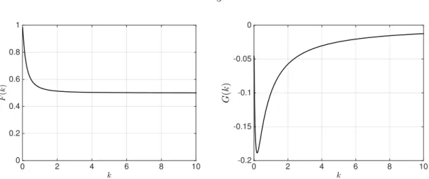
1.1 Real,F(k), and Imaginary,G(k), part of the Thedorsen’s function,C(k). . . 5 1.2 Fluctuating amplitude (left) and phase (right) of lift relative to velocity. The results

of Greenberg’s model (Greenberg, 1947) and the discrete-vortex model (DVM) from Tchieu & Leonard (2011) are presented. . . 6

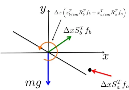
2.1 Flow diagram of the gradient-based optimization procedure, and a comparison of the convergence of conjugate gradient method (red line) with steepest decent method (green line). . . 21 2.2 Free body diagram of an airfoil with a actuator near the trailing edge. Gravity and

resultant fluid force are depicted. . . 25

3.1 Hopf bifurcation at Recrit = 254 (simulation). Fluctuating ranges (gray area) and mean values (dashed line) are shown for 250<Re <290. Flat plate,α= 15^◦. . . 36 3.2 Critical Reynolds numbers (Recrit) and corresponding vortex shedding reduced fre-

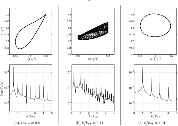
quencies (kvs, crit) at different angles of attack. The subscriptp refers to quantities made dimensionless by the projected chord length,csinα. . . 36 3.3 Representative cases with (left and right) and without (center) lock-in. Surging ampli-

tude isσx = 0.05 and the phase plot of lift coefficient and x-velocity are shown with the frequency spectra for 50 periods of surging frequency, k. Flat plate, Re = 300, α= 15^◦ andkvs = 1.62. . . 38 3.4 Lock-in regions (left) and mean lift force (right) for a surging airfoil atRe= 300 and

α= 15^◦. Lock-in regions are defined whereγ <10⁻². L0is the mean lift forσx= 0. . 39

(11)

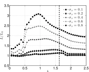
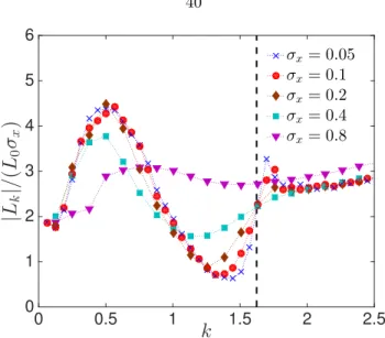
3.5 Time-averaged lift for 0.1 < σx < 0.8. Vertical line indicates the vortex shedding frequency of steady flow (σx= 0). Flat plate,α= 15^◦,Re= 300. . . 39 3.6 Fluctuating amplitude of lift. Aerodynamic response is nearly independent ofσx for

σx≤0.2. Vertical line indicates the vortex shedding frequency of steady flow (σx= 0).

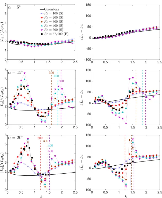
Flat plate,α= 15^◦,Re= 300. . . 40 3.7 Amplitude (left) and phase (right) of the fluctuating lift at various Re and α. Sim-

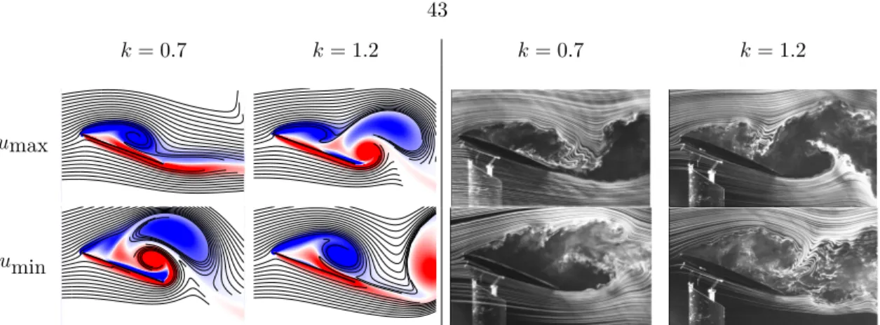
ulation results (S), Re ∈ [100,500], are compared with the experiment results (E), Re = 57,000. Vertical lines indicate the vortex shedding frequency of steady flow (σx = 0) at corresponding Re. Airfoil is a flat plate for the simulations and NACA 0006 for experiments. σx was set to 0.1 for all cases. . . 42 3.8 Snapshots of flow field atRe = 500 (left, simulation) andRe = 57,000 (right, experi-

mental) for α= 20^◦ and σx = 0.1. Top and bottom rows correspond to the flow field at the maximum u=U(1 +σx) and minimum u= U(1−σx) velocity, respectively.

Reduced frequencies are chosen to reveal flow fields when the fluctuations are amplified (k= 0.7) and attenuated (k= 1.2). For the simulations, streaklines are depicted on top of the color contours of vorticity,ωc/U ∈[−10,10]. . . 43 3.9 Vorticity contours and velocity vectors at various Reynolds number. Left and right

columns shows the flow field at the maximum u = U(1 +σx), and minimum u = U(1−σx) velocity, respectively. α= 15^◦, σx= 0.2 andk= 0.5. . . 44 3.10 Same as figure 3.9 but atk= 1.26. . . 45 3.11 Strength of maximum shed LEV and its occurring phase. Snapshots reveal the strength

and size decreasing with increasing k. Flat plate, α = 15^◦, Re = 300 and σx = 0.2.

ωc/U ∈[−10,10]. . . 47

(12)

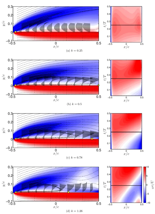
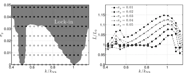
3.12 Streamlines (dashed lines), streaklines (solid lines), and stagnation points (diamond symbols) on the upper surface are plotted on top of vorticity contours at the maximum velocity,u=U(1 +σx), fork= 0.25,0.5,0.78,and 1.26. For each case, vorticity values on the upper surface during the advancing portion of the motion are plotted on the right. Flat plate, Re = 300, α = 15^◦, and σx = 0.2. ωc/U ∈[−10,10]. Flat plate is rotated 15^◦ to align its chord with the x-axis. . . 49 3.13 Lock-in regions (left) and mean lift force (right) forRe = 300 andα= 15^◦. L0 is the

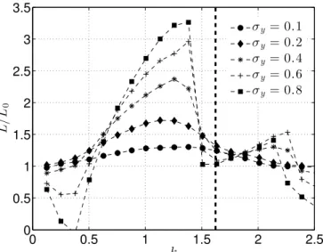
mean lift forσy= 0. . . 50 3.14 Time-averaged lift for 0.1 < σy < 0.8. Vertical line indicates the vortex shedding

frequency of steady flow (σy= 0). Flat plate,α= 15^◦,Re= 300. . . 51 3.15 Fluctuating amplitude of lift at various reduced frequencies, k. Flat plate, α= 15^◦

andσy = 0.05. . . 52 3.16 Fluctuating amplitude of lift (plunging). Aerodynamic response is nearly linear for

σy = 0.2. Vertical lines indicate the vortex shedding frequency of steady flow (σy = 0).

Flat plate,α= 15^◦,Re= 300. . . 53

4.1 The square box near the leading edge is enlarged to show control volume geometry (region inside the dotted line) and vorticity flux ofω <0 through the control surface.

Flat plate,α= 20^◦,k= 0.5,σ= 0.4 atRe= 1000. . . 57 4.2 Lift spectrum of uniform flow atα= 20^◦. ˆCL is the magnitude of the Discrete-Fourier

Transform of the fluctuating lift coefficient. The red dashed line corresponds to a frequency ofStvs =f csinα/U = 0.2. . . 58 4.3 Time history of lift coefficient atRe= 100,500, and 1000. . . 59 4.4 Mean drag (left) and lift (right) coefficients of uniform flow atα= 20^◦. . . 59

(13)

4.5 Time-averaged lift coefficient, ¯CL, of streamwise oscillating flow at various reduced frequencies (α = 20^◦). Simulation (S) are run at Re = 1000 and compared with experimental data (E) from Gursul & Ho (1992),Re = 5×10⁴. Dashed line corresponds to the frequency of maximum lift of experiment results (atk= 0.8). The time-averaged lift coefficient of uniform flow atRe= 1000 is ¯CL0= 1.15. . . 60 4.6 Snapshots of flow fields at Re = 1000 (top, simulation) and Re = 50,000 (bottom,

experimental) forσx= 0.7. The reduced frequencies for the simulation and experiment are k = 0.75 and k = 0.7, respectively. The maximum velocity, umax =U(1 +σx), occurs att/T = 0.25 and the minimum velocity, umin = U(1−σx), att/T = 0.75.

Vorticity contours and streamlines are compared to experimental flow visualizations (Gursul & Ho, 1992). ωc/U ∈[−20,20]. . . 61 4.7 Time history of lift coefficient, CL, for 2 oscillating periods of the motion. Increasing

sequence of reduced frequency fromk= 0.25 tok= 0.75. u⁰ is the fluctuating velocity of the airfoil’s motion. α= 20^◦,Re = 1000, andσx= 0.4. . . 64 4.8 Corresponding flow field of figure 4.7. ωc/U ∈[−20,20]. . . 65 4.9 LEV formations during the advancing period. α= 20^◦,Re= 1000 andσx= 0.4. . . . 66 4.10 The dynamic formation time, Tdf, at various σx. The dynamic formation time is

measured from the start of the advancing phase, i.e.,t0= 0. . . 67 4.11 LEV formation time,T^∗, is measured at various reduced frequencies (blue circle line).

The formation time evaluated using the period of the motion,π/k, is also shown as the upper bound (black solid line). Flat plate,α= 20^◦ andσ= 0.4 atRe= 1000. . . 68 4.12 Total and max LEV circulation at various reduced frequencies. Flat plate, α= 20^◦

andσ= 0.4 atRe = 1000. Circulation is non-dimensionalized as Γ^∗ = Γ/U c. For the range of 0.38< k <1, the LEV is grown to its maximum strength and the rest of the total vorticity is analogous to the vortices in the trailing jet in the vortex ring case (Gharibet al., 1998). . . 69

(14)

4.13 Flow fields shown as a series of increasing convective time,tU/c, fork= 0.25,k= 0.5, andk= 0.75. Time is measured from the start of the advancing motion. Left and right pointed arrows indicate the advancing and retreating portion of the period, respectively.

Double horizontal line is associated with the LEV formation time, which occurs at 3 < T^∗ < 4. Single horizontal line indicates the end of one period of the motion.

α= 20^◦,Re = 1000, andσx= 0.4. . . 70 4.14 Same as figure 4.13, but atk= 1, 1.25, and 2.01. . . 71 4.15 Sinusoidal and square waveform of streamwise velocity. σx= 0.4. . . 72 4.16 Time-averaged lift coefficient, ¯CL. Black solid line shows the result obtained using the

square waveform streamwise velocity. . . 73 4.17 Time history of lift coefficient at various reduced frequencies. Only the advancing

portion of the period, 0< t/T <0.5, is shown. . . 74 4.18 Same as figure 4.19, but with square waveform of streamwise velocity. Results are

shown atk= 0.25, 0.5, and 0.63. . . 75 4.19 Same as figure 4.19, but with square waveform of streamwise velocity. Results are

shown atk= 0.75, 1, and 1.51. . . 76

5.1 Schematic of the test problem. Flat plate moving at a constant velocity,U, with the rotational axis located 0.3 chord length from the leading-edge. Ω is the angular velocity of the body. . . 79 5.2 Drag and lift coefficient of uniform flow at various angles of attack. Shaded region shows

the range of values, and the dash line, the average. Flat plate,Re= 500. Aerodynamic forces measured at every 2^◦. Transition from a stable equilibrium to periodic vortex shedding occurs at 10^◦. . . 79

(15)

5.3 Optimization results of a flat pate atα= 0^◦ (black),15^◦ (red), 30^◦ (green), and60^◦ (blue). Angle of attack (left) and lift coefficient (right) is plotted as a function of time.

Dashed line indicates the case before control and solid line, after. Optimization leads the airfoil to rotate towards the angle that maximizes lift, which is near 45^◦. Control time horizon,T, is 40 convective time units. . . 80 5.4 Flapping motion of a wing element in 2D. Downstroke phase indicated by the dotted

line and upstroke by the solid line. The stroke plane is inclined at an angleβ, with an amplitude ofA0. ais the distance of the rotating axis from the leading edge, and α, the pitch angle. . . 83 5.5 Flapping motions before (left) and after (right) optimization. . . 84 5.6 Vorticity field of the optimized wing motion atβ= 0^◦. . . 85 5.7 Time history of the vertical force coefficient, Cy, for the optimized result of β = 0^◦.

Dashed line indicates the data before optimization, and solid line, after. Shaded region indicates the stroke moving from right to left. . . 86 5.8 Time history of power,P, for the optimized result ofβ = 0^◦. Shaded region indicates

the stroke moving from right to left. . . 87

A.1 Coordinate systems of fixed (inertial) and (non-inertial) rotating frame or reference. . 92

B.1 Checkpointing algorithm developed by Wanget al.(2009). Evolution of the algorithm assuming a total of 25 time steps. 5 checkpoints are assigned to save the forward variables. Copyright c2009 Society for Industrial and Applied Mathematics. Reprinted with permission. . . 96

(16)

List of Tables

5.1 Summary of optimization results. ¯CL is the time-averaged lift coefficient after control, and ¯CL0 before. The integrated control cost is defined as RT

0 QRΩ²dt, and reference lift coefficient normalized asCL,ref= 2FL,ref/ρU²c. T is the control horizon. . . 81 5.2 Summary of optimization results. A0 = 2.5c, a = 0.3c, and Re = 100 for all cases.

Time-averaged normalized forces, ¯Cx= 2Fx/(ρU²c), and ¯Cy = 2Fy/(ρU²c), in the x and y direction are given, respectively. Time-averaged power is also presented in the table, where ¯P includes both the rotational and translational power. The subscript with 0 indicates the values for cases before optimization. Control horizon,T, is set to 40 convective time units, which is close to 5 flapping period. . . 84

(17)

Nomenclature

A peak-to-peak amplitude of unsteady airfoil motion

CD drag coefficient

CL lift coefficient

Lam added mass lift

Lqs quasi-steady lift

L0 mean lift at a constant velocity

L¯ mean lift

Lˆk magnitude of Fourier coefficient of lift at frequencyk

Re Reynolds Number, (cU/ν)

Recrit Critical Reynolds Number

Stc Strouhal number scaled with airfoil chord length (f c/U) StA Strouhal number scaled with peak-to-peak amplitude (f A/U) T Period of oscillation or control time horizon

Tdf dynamic formation time T^∗ universal formation time

U reference velocity

c airfoil chord length

k reduced frequency, (πf c/U =πStc)

kvs reduced frequency corresponding to vortex shedding

kvs, crit reduced frequency corresponding to vortex shedding atRecrit u streamwise airfoil velocity

(18)

v transverse airfoil velocity x0 center of rotation

Γ circulation

Ω angular velocity

α angle of attack

ν fluid kinematic viscosity

ρ fluid density

σx amplitude of oscillating streamwise velocity with respect to the reference velocity σy amplitude of oscillating transverse velocity with respect to the reference velocity φ phase of lift leading velocity

ω vorticity

DVM Discrete vortex model

IBFM Immersed boundary fractional step method

LEV Leading-edge vortex

MAV Micro-air vehicle TEV Trailing-edge vortex

(19)

Chapter 1

Introduction

As a new class of air vehicles that operate at low Reynolds number, micro-air vehicles (MAVs) face unique challenges different from conventional aircraft. In this low Reynolds number regime, air vehicles are exposed to high drag coefficients (CD), due to laminar flow separation. For their small size and low flight speed, encountering a gust leads to a unsteady flow field, and in some occasions, to stall. Furthermore, transitions from steady to unsteady flow and from laminar to turbulent flow are a frequently encountered phenomenon that conventional aircraft do not experience.

Perhaps for these reasons, birds have adapted to fly with agility at low Reynolds number by utilizing flapping wings (Dickinson & Gotz, 1993; Ellington et al., 1996; Wang, 2005; Pesavento &

Wang, 2009).

Regardless of whether a wing is flapping or steadily translating through a gusting flow, better understanding of unsteady aerodynamics at low Reynolds number is required to design efficient and effective MAVs. In this study, we identify distinct features of unsteady flows at low Reynolds number, and implement an optimal control strategy for controlling aerodynamic forces in unsteady flow.

(20)

1.1 Energy extraction and unsteady aerodynamics at low Reynolds number

Birds have evolved to efficiently transfer energy from the surrounding environment to improve their flight performance and maneuverability. An albatross exploits energy from the velocity gradients of the oceanic boundary layer through dynamic soaring (Denny, 2009), and numerous kinds of birds take advantage of the spatial and temporal gradients of the atmospheric gust to remain aloft without flapping their wings. Extracting energy from the atmospheric gusts during its migration, an Alpine swift is known to continue its journey for 200 consecutive days without being on the ground or in water (Liechtiet al., 2013). Thermals and the upward drafts created by the topology also provide additional sources of energy (Weimerskirchet al., 2003).

Recently, there have been several attempts to understand the coupling between the flight mechanics and the underlying fluid dynamics to improve unsteady flight performance of unmanned or micro-air vehicles. Lissaman (2005) considered small vehicles whose flight speed is comparable to atmospheric wind variations. The lift-to-drag ratio was found to be the primary parameter for achieving neutral energy cycles for a vehicle flying through a sinusoidal vertical gust (Lissaman &

Patel, 2007), and a state feedback controller that measures current wind speed and its gradient has shown energy gains for both sinusoidal and turbulent gusts (Langelaan, 2009). However, in each of these studies, the models were based on quasi-steady flow approximations where the forces are determined by the instantaneous state of the flow through a static map. Recent studies, discussed more fully below, cast doubt upon this approximation.

While classical unsteady potential flow models effectively describe the dynamical effects on fluid forces through the added mass and trailing-edge Kutta condition (Theodorsen, 1935; Von Karman &

Sears, 1938; Greenberg, 1947; Tchieu & Leonard, 2011), these cases are restricted to small changes in velocity at low angle of attack and high Reynolds number, and no comprehensive theory is available for higher angles when the flow separates. MAVs, in particular, are vulnerable to flow separation since laminar boundary layers are less resistant than turbulent boundary layers to the

(21)

adverse pressure gradient, and small scaled vehicles would experience separations more frequently than conventional aircraft.

Unsteadiness in conventional air vehicles is considered a deficit since the unsteady motion can lead to separation, instabilities, and flow-structure interactions that are difficult to control. However, with clear understanding of the flow, unsteady effects associated with separations can be utilized to improve maneuverability and performance of MAVs (Pesavento & Wang, 2009). The unsteady motion associated with the flapping flight of insects and birds produces much higher lift than the corresponding steady case (Ellington et al., 1996), and a number of studies have focused on this topic to understand the corresponding flow structures (Dickinson & Gotz, 1993; Ellington et al., 1996; Wang, 2005; Pesavento & Wang, 2009), that could be potentially useful for MAVs. The presence of a leading-edge vortex (LEV) was found to be essential for providing sufficient lift in insect flight (Dickinson & Gotz, 1993; Ellingtonet al., 1996), and the aerodynamic power required in flapping motions was reduced by capturing its own wake that was generated in the previous stroke cycle (Pesavento & Wang, 2009). Williams et al. (2011) have also shown that combining vertical motions of an airfoil with a streamwise oscillating gust produces a net energy gain of the airfoil that is positive when the lift and drag fluctuations are large enough.

The interaction between the wing and the previously shed vortices, sometimes termed ‘wake capture’ when the wing exploits energy from the shed vortices, is also a mechanism to enhance lift. The shed LEV may immediately move far from the wing without causing any notable changes to the force history, or stay close to the airfoil so that the airfoil can take advantage of the low pressure region that is induced by the LEV. For instance, at the end of each forward and backward stroke, fruit flies are known to gain sufficient lift from the lingering wake that was generated from the previous stroke (Dickinsonet al., 1999).

For MAVs at high-angles of attack, large-scale vortices associated with separation, such as the LEV or the dynamic-stall vortex, significantly alter the behavior of the aerodynamic forces. Gursul

& Ho (1992) and Gursul et al. (1994) examined a NACA 0012 airfoil immersed in a temporally varying freestream, and the peak time-averaged lift occurred at a frequency associated with the

(22)

shed LEV inducing high pressure gradients normal to the wing during the retreating portion of the cycle. A similar time-averaged behavior of lift has been investigated for transverse airfoil motions (Andro & Jacquin, 2009; Calderon et al., 2013; Cleaveret al., 2011, 2013), and the peak occurred at a frequency where the shed LEV remained close to the airfoil during its convection.

The structure of the LEV over a pitch / surge combined motion has also been investigated by Tsai & Colonius (2015) and Dunne & McKeon (2015) on a two-dimensional vertical-axis wind turbine. Tsai & Colonius (2015) observed that the vortex pair that traveled along with the airfoil substantially decreased lift in the presence of the Coriolis force. For an equivalent planar motion (without the Coriolis effect), the growth and separation of the LEV were described by the interactions of the primary and secondary dynamic separation modes that corresponded to the first and second harmonic frequencies of the motion (Dunne & McKeon, 2015).

1.2 Flow models of unsteady aerodynamics

When the flow is attached, classical potential flow models can be utilized to effectively describe the aerodynamic forces of a moving airfoil. Theodorsen (1935) was one of the pioneers to develop an unsteady potential model in 2D to predict the aerodynamic loads on a fluttering airfoil. The main assumptions of his approach are as follows:

• Flow is considered at high Reynolds number flow, and the viscous effects neglected.

• Fluttering amplitude and frequency of the thin airfoil are small enough such that the flow remains attached throughout the entire motion.

• The separation point is only at the trailing edge of the airfoil, and the amount of vorticity in the wake is determined by satisfying the Kutta condition.

• The wake convects with the same speed as the freestream velocity.

(23)

k

0 2 4 6 8 10

F(k)

0 0.2 0.4 0.6 0.8 1

k

0 2 4 6 8 10

G(k)

-0.2 -0.15 -0.1 -0.05 0

Figure 1.1: Real, F(k), and Imaginary,G(k), part of the Thedorsen’s function,C(k).

With these assumption, the lift coefficient,CL, of a thin flat plate under harmonic plunging and pitching can be expressed as,

CL= π 2

−¨yb−x0α¨+ ˙α

| {z }

CAM

L

+C(k) 2π

α−y˙b + 1

4−x0

˙ α

| {z }

CQS

L

, (1.1)

where, x0 is the pitch axis location respect to the mid-chord (pitching about the leading edge corresponds tox0=−0.5, whereas the trailing edge is atx0= 0.5), andyb the transverse movement of the airfoil. The equation is nondimensionalized by normalizing length, velocity, and time by the chord length, c, freestream velocity, U, and convective time unit, c/U, respectively. The first term of equation 1.1 correspond to the non-circulatory part of lift due to the reaction forces of the ambient fluid being accelerated (known as the added mass). The second term accounts for the bound circulation that is induced by the wake vortices. The Theodorsen function, C(k) =F(k) +iG(k), which is solely a function of the reduced frequency, k = πf c/U, can be understood as a transfer function that attenuates and lags the phase of lift by an amount that depends on the frequency of the oscillations. Figure 1.1 plots the real and imaginary part of C(k) as a function of the reduced frequency. In the limit of k going to zero and infinity,CL asymptotically reaches the quasi-steady value,CQS

L , and the added mass liftCAM

L , respectively.

(24)

k

0 1 2 3 4 5

| ˆ C

L

| / ( C

L0

σ

x

)

0 0.5 1 1.5 2 2.5 3 3.5 4

Greenberg DVM

k

0 1 2 3 4 5

φ

x

-20 0 20 40 60 80

Figure 1.2: Fluctuating amplitude (left) and phase (right) of lift relative to velocity. The results of Greenberg’s model (Greenberg, 1947) and the discrete-vortex model (DVM) from Tchieu & Leonard (2011) are presented.

Greenberg (1947) extended Theodorsen’s model to include the effects of an oscillating freestream on the unsteady lift. With pure freestream oscillation ofU_∞=U(1 +σxsinωxt), the lift coefficient in Greenberg’s formula can be derived as,

CL

CL0 = 1 +σx



sk 2 +G

2

+ (1 +F)²





| {z }

CˆL(k)

sin (ωxt+φx) +O(σ²_x), (1.2)

φx= tan⁻¹

(k

2 +G)/(F+ 1)

. (1.3)

In equation 1.2, the instantaneous lift coefficient is normalized by the quasi-steady lift coefficient, CL0 = 2πα, and high order terms are neglected for σx 1 (otherwise the flow would not stay attached). According to this model, the time-averaged lift remains independent ofk; however, the fluctuating amplitude and phase of lift are greatly effected by the reduced frequency. Figure 1.2 plots the normalized amplitude and phase of lift relative to the freestream velocity. CˆL is the Fourier component of the fluctuating lift coefficient at the corresponding oscillating frequency, k.

Note that the normalized amplitude,|CˆL|/(CL0σx), and phase of lift, φx, are solely a function of k, and interestingly, the fluctuations are minimized near a frequency ofk= 0.8.

(25)

In a similar fashion, the lift coefficient of a plunging airfoil, uy =U σysin (ωyt), with constant freestream velocity,U_∞=U, can be derived as,

CL

CL0

= 1 +σy

α



 skx

2 +G ²

+F²



sin (ωyt+φy) +O(σ²_y), (1.4)

φy= tan⁻¹

(k

2 +G)/F

. (1.5)

Using the basic concepts of vortex theory, Von Karman & Sears (1938) derived a formula similar to Theodorsen’s model (Theodorsen, 1935), avoiding the complicated mathematical derivations that previous studies possessed. With the same assumptions given as in the Theodorsen’s model, they were able to compute the aerodynamic loads on oscillating airfoils as well as on sharp-edge gusts.

Recently, Tchieu & Leonard (2011), assuming discrete vortices in the wake rather than a continuous distribution of vorticity, developed a discrete version of the Von Karman & Sears (1938) model, which in this study is referred to as the discrete vortex model (DVM). The nascent vortex moves at a speed that satisfies the Brown and Michael equation (Brown & Michael, 1954), and sheds whenever it reaches its maximum strength. After the vortex is shed, it convects as the same speed as the freestream velocity. Along with Greenberg’s formula, the fluctuating lift coefficient of DVM for the case of streamwise varying velocity is shown in figure 1.2. Despite the convecting speed of the nascent vortex and the discretization of the wake, most of the assumptions that are used to con- struct the DVM are the same as for the Greenberg’s model, and the results are similar. In chapter 3, the lift coefficient obtained from these models will be compared with equivalent computational and experimental results of attached and separated flows.

Although classical unsteady flow models effectively compute the fluid forces on a airfoil (Theodorsen, 1935; Von Karman & Sears, 1938; Greenberg, 1947; Tchieu & Leonard, 2011), the assumptions of the models restrict the flow to be valid only at low angles of attack, high Re, and small changes of amplitude in motion. For MAVs that operate at high angles of attack and low Re, viscous effects are no longer negligible, and the flow around the airfoil experiences separation more frequently. At present, no comprehensive theory is available for a fully stalled flow; however, many studies have

(26)

attempted to develop a model that covers a wider range of flows than the classical flow models.

Enforcing a Kutta condition also at the leading edge, low-order point vortex models have been developed to additionally include the contribution of a LEV on the aerodynamic forces (Wang &

Eldredge, 2013; Darakanandaet al., 2016). The full description of an inviscid model with multiple Kutta conditions is beyond the scope of this study, and we recommend the reader to refer to Hemati et al.(2014) and Darakanandaet al. (2016) for further details.

The process of a dynamic stall, in general, occurs on a smaller time scale than the development of a full stall (Wang & Eldredge, 2013), and the transient response of the fluid forces to the airfoil motion above the stall angle have also been studied extensively. Related models that are associated with lowRe forward and flapping flights are summarized by Tahaet al. (2014).

1.3 Application to flow control problems

Depending on whether the system requires the input of energy, flow control strategies can be cat- egorized as either passive or active. Passive control devices modify the geometry of the surface to satisfy a control objective. Among many passive devices, dimples (Bearman & Harvey, 1993; Choi et al., 2006), splitter plates (Anderson & Szewczyk, 1997), riblets (Bechertet al., 2000), and spoilers (Beaudoin & Aider, 2008) are the successful examples that reduce drag or enhance stability. How- ever, there is no systematic way to design devices that meet a given objective, and their shape must be determined through laborious experiments on numerous prototypes.

Active control, on the other hand, requires energy input of the system by the actuator. Whether the output of the system is fed back to the input or not, active control can be classified as either open-looporclosed-loop control (passive control devices are open-loop controllers). Active open-loop control uses various forcing devices that control the motion of the body (Tokumaru & Dimotakis, 1991) or effectively change the flow around the body (Wu et al., 1998; Greenblatt & Wygnanski, 2000; Post & Corke, 2006). As for passive control methods, a deep understanding of the flow system is required to obtain successful control outputs.

Recently, there has been more interest in closed-loop active control methods, whereby the ac-

(27)

tuator (input) is continuously modified by the response of the system. Closed-loop control has an advantage over open-loop control in terms of stability, because it is less sensitive to disturbances and uncertainties. Feedback control using proportional-integral-derivative controllers (Zhanget al., 2004) as well as reduced-order models (Ahuja & Rowley, 2010) has been successfully applied to nonlinear unstable flow problems. Kerstenset al.(2011) also applied closed-loop control to suppress lift fluctuations in an unsteady freestream. Feedback control, in general, performs better than open- loop control systems, but, in nonlinear fluid problems, it is sometimes difficult to choose the best feedback signal that enhances the performance.

The feedback control approach used in this study is adjoint-based optimal control, where the control inputs that minimize a cost function are determined, under the constraint that the dynamics satisfy the governing differential equations. Adjoint variables are introduced as Lagrange multipliers enforcing the system to satisfy the constraint equations. With an initial guess of the control inputs, this method finds the optimal control that locally minimizes the cost over a given time horizon, T. One advantage of this method, numerically, is that the computational cost to compute the gradient does not increase with the number of controls. For example, Bewley et al. (2001) used every point in the flow domain as an actuator for blowing and suction, re-laminarizing a turbulent channel flow. Unlike other passive and active control approaches, optimal control does not require a priori knowledge of the physical mechanism that minimizes the cost, and the optimal solutions themselves often illuminate aspects of the underlying flow physics that would not otherwise have been appreciated.

Currently, due to their high computation cost, adjoint methods are considered as an offline optimization scheme. However, in the future, the development of high performance computers and efficient numerical tools will reduce the time required to compute the solutions, and the adjoint method can perform as a real-time feedback controller. Also, as with the development of lidar (a radar that uses light from a laser) that is capable of measuring upstream flows (Schmittet al., 2007), the adjoint method can provide estimates of best or worst control strategies during aviation. The further the laser sensor can measure upstream, the further we are capable of predicting the future

(28)

with long-term control strategies.

Adjoint based control also arises in shape optimization problems. Pioneered by Jameson (1988), efforts to find the airfoil geometry that minimizes a given cost function were conducted by various researchers (Reutheret al., 1999; Gileset al., 2003). The primary goal in most of these studies was to maximize the lift-to-drag ratio,L/D, as a measure of the aerodynamic efficiency. Nevertheless, these cases were limited to high Re and low angle of attack, where the aerodynamic forces were highly effected by the airfoil geometry. For unsteady motions of an airfoil at low Re, owing to the fact that viscous effects are more severe and flows being more vulnerable to separation than higher Re flows, aerodynamic forces are less sensitive to the change of airfoil geometry. AtRe∼10²−10³, viscous effects are relatively large, causing high drag and limitingL/Dto be an order of magnitude less than higherRe(>10⁵) cases (Lissaman, 1983). Insects flap their wings at high angles of attack (α >30^◦), and the flows around their wings are likely to be separated. As a consequence, airfoil shape optimization in lowRe flights may not guarantee the promising results obtained at highRe cases. Instead, for unsteady flows at lowRe, finding the optimal parameters of the airfoil’s motion (kinematic optimization) may be a better strategy to achieve high aerodynamic performance.

1.4 Thesis outline

In chapter 2, we discuss the numerical method used to solve unsteady, incompressible flows around airfoils at low Reynolds number, and derive equations for implementing optimal control. In addition, numerical subtleties such as discrete operators, multi-grid techniques, checkpointing algorithms, conjugate gradient method, and line minimization are as well discussed.

In chapter 3, the flow structure and the aerodynamic forces associated with small-amplitude streamwise (surging) and transverse (plunging) oscillating of an airfoils at low Reynolds number are investigated. For simplicity, two-dimensional flows are simulated and we restrict the Reynolds number toO(10²−10³) such that, depending on the specific values of angle of attack and Reynolds number, the flow can be subcritical, steady flow, or supercritical, with respect to the usual wake instability associated with a bluff body. The mean and fluctuating behavior of the aerodynamic forces

(29)

associated with vortical structure of the wake (vortex lock-in, LEV) are discussed and compared with the experimental results.

High-amplitude surging motions are considered in chapter 4. As the variation in the Reynolds number associated with the motion is large, non-oscillatory uniform flows are first investigated over a wide range of Reynolds number. For the high-amplitude surging motions, the mechanism that leads to the time-averaged peak of lift is of a particular interest, and we investigate this problem by examining vortex strength and flow fields. The time-averaged lift of a motion with square-wave streamwise velocity is also investigated to understand the flow behaviors that are associated with high accelerations.

In chapter 5, using the optimal control framework developed in chapter 2, a simple example that obtains the optimal angle of a flat plate that maximizes lift is presented as a test problem. Optimal control is also applied to flapping motions, where the optimized motion resembles that of a flying insect.

(30)

Chapter 2

Numerical Methods

The immersed boundary fractional-step method (IBFS), which is used as our fluid solver, is described.

Optimal control theory using adjoint equations is also introduced, and used to compute the gradients of the design parameters that minimize a predefined cost function.

2.1 Immersed boundary fractional step method

The immersed boundary fractional-step method (IBFS) (Taira & Colonius, 2007; Colonius & Taira, 2008) has been used to solve a two dimensional incompressible flow in the (non-inertial) reference frame of the body (appendix A). The method solves the vorticity-streamfunction formulation of the Navier-Stokes equations and the body is represented by a discrete set of (regularized) surface forces to enforce the no-slip condition. We review the derivations by considering the continuous version of the incompressible Navier-Stokes equations with boundary force,f, and no-slip condition (Peskin, 1972, 2002):

∂u

∂t +u· ∇u=−∇p+ 1

Re∇²u+ Z

s

f(ξ(s, t))δ(ξ−x)ds, (2.1)

∇ ·u= 0, (2.2)

u(ξ(s, t)) = Z

x

u(x)δ(x−ξ)dx=ub(ξ(s, t)). (2.3)

The convolutions with the Dirac delta function, δ, are used to exchange information between the Eularian fluid grid and the Lagrangian body points. Discretizing the above equations, using the

(31)

Adams-Bashforth 2nd order scheme on advection term and the Crank-Nicolson method on viscous term (Taira & Colonius, 2007), the terms can be collected to form a matrix such as:







Aˆ Gˆ −Hˆ Dˆ 0 0 Eˆ 0 0











 uⁿ⁺¹

φ f∆t







=





 ˆ rⁿ

0 uⁿ⁺¹_B





 +





 bcˆ1

bc2

0







, (2.4)

where

Aˆ≡I−∆t

2 Lˆ and ˆrⁿ≡

I+∆t 2 Lˆ

uⁿ−3∆t

2 N(uˆ ⁿ) +∆t

2 Nˆ(uⁿ⁻¹). (2.5)

Here, ˆGand ˆDare the discrete gradient and divergence operator, respectively. The regularization ( ˆH) and interpolation ( ˆE) operators smear the immersed forces over a few cells and interpolate velocities back to the Lagrangian body points with the specific form of delta function designed by Roma et al. (1999). ˆL is the standard 5-point stencil 2nd order Laplacian operator and ˆN the operator relating to the nonlinear term.

Introduce the scaling operatorsR and ˆM:

R≡







∆yj 0 0 ∆xi





 and Mˆ ≡







1

2(∆xi+ ∆x_i−1) 0 0 ¹₂(∆yj+ ∆y_j−1)





 . (2.6)

equation (2.4) can be written as:







A G −H

D 0 0

ERˆ ⁻¹ 0 0











 qⁿ⁺¹

φ f∆t







=





 rⁿ

0 uⁿ⁺¹_B





 +





 bc1

bc2

0







, (2.7)

(32)

where

A≡MˆARˆ ⁻¹, G≡MˆG, Hˆ ≡MˆH,ˆ

D≡DRˆ ⁻¹=−G^T, rⁿ≡Mˆrˆⁿ, bc1≡Mˆbcˆ1, andqⁿ⁺¹≡Ruⁿ⁺¹.

Also, the mass matrix and the Laplacian are additionally defined as M ≡ M Rˆ ⁻¹ and L ≡ MˆLRˆ ⁻¹such thatA=M−^∆t₂ L. We note thatAis symmetric and positive-definite by construction.

For the null space approach in Colonius & Taira (2008), the vorticity-streamfunction formula of the Navier-Stokes equation is solved instead of the primitive variables on a uniform Cartesian grid. The discrete streamfunction, s, is used that satisfies q=Cs. C represents the discrete curl operator, which is constructed with column vectors corresponding to the basis of the null space of D. Therefore, these operators enjoy the following relation:

DC ≡0, (2.8)

which mimics the continuous identity ∇ · ∇× ≡0.

We also introduce another discrete curl operation,C^T, that is defined as,

γ=C^Tq , (2.9)

which is a second-order accurate approximation of the circulation in each dual cell. For the Laplacian,

Lq=− 1

Re∆x²CC^Tq=− 1

Re∆x²Cγ≡ −βCγ , (2.10)

provided that Dq = 0, where β = _Re∆x¹ 2. This identity mimics the continuous identity ∇²u=

(33)

∇(∇ ·u)− ∇ × ∇ ×u=−∇ × ∇ ×u.

Taking the curl of the momentum equation, which we multiplyC^T at both sides of the equation in the first row of the matrix in equation (2.7), the pressure variable is eliminated (C^TG=−(DC)^T = 0) and the incompressible constraint is automatically satisfied. The matrix form can be rewritten in the following form:







I+^β₂∆tC^TC C^TEˆ^T EC(Cˆ ^TC)⁻¹ 0











 γⁿ⁺¹

f∆t





=





 C^Trⁿ uⁿ⁺¹_B ∆x





+







β∆t bcγ

0





 . (2.11)

Decomposing the left-hand side matrix into a Lower and Upper triangular matrix (Perot, 1993),

LU =







I+^β₂∆tC^TC C^TEˆ^T EC(Cˆ ^TC)⁻¹ 0





 (2.12)

the corresponding matrices are,

L=







I+^β₂∆tC^TC 0

EC(Cˆ ^TC)⁻¹ −EC(Cˆ ^TC)⁻¹

I+^β₂∆tC^TC−1

C^TEˆ^T





, (2.13)

U =







I

I+^β₂∆tC^TC−1

C^TEˆ^T

0 I





. (2.14)

We first solve,

L





 γ^∗

f





=





 C^Trⁿ uⁿ⁺¹_B ∆x





+







β∆t bcγ

0





, (2.15)

(34)

which leads to the equation,

S

I+β∆t 2 Λ

Sγ^∗=C^Trⁿ

=

I−β∆t 2 C^TC

γⁿ+ ∆t 2∆x²

3C^TN(q^(k)ⁿ)−C^TN(q^(k)ⁿ⁻¹)

+β∆t bcγ. (2.16)

The matrixC^TCis now diagonalized with discrete sin transformC^TC=SΛSfor computational efficiency. To implement the multi-domain technique, equation (2.16) will be modified so thatγ^∗ is now computed on a progressively coarsifying grids with the corrected boundary condition (Colonius

& Taira, 2008):

S

I+β∆t 2 Λ

Sγ^(k)^∗=S

I−β∆t 2 Λ

Sγ^(k)ⁿ+ ∆t 2∆x²

3C^TN(q^(k)ⁿ)−C^TN(q^(k)ⁿ⁻¹)

+β∆t 2 bcγ

[P^(k+1)^→^(k)(γ^(k+1)^∗)] + [P^(k+1)^→^(k)(γ^(k+1)ⁿ)]

(2.17)

=⇒ γ^(k)^∗=S

I+β∆t 2 Λ

−1 S

3∆t

2∆x²C^TN(q^(k)ⁿ)− ∆t

2∆x²C^TN(q^(k)ⁿ⁻¹) +β∆t

2 bcγ

[P^(k+1)^→^(k)(γ^(k+1)^∗)] + [P^(k+1)^→^(k)(γ^(k+1)ⁿ)]

+

I−β∆t 2 Λ

Sγ^(k)ⁿ

. (2.18)

Then we solve for the immersed boundary forces, f, by computing the second row of the equation 2.15.

ECˆ SΛ⁻¹

I+β 2Λ

−1

S

!

C^TEˆ^Tf∆t= ˆECSΛ⁻¹Sγ^∗−uⁿ⁺¹_B ∆x (2.19)

=⇒ f∆t= ECSΛˆ ⁻¹SS

I+β 2Λ

−1

SC^TEˆ^T

!−1

ECSΛˆ ⁻¹Sγ^∗−uⁿ⁺¹_B ∆x

. (2.20)

If the body is not moving with respect to the grid, Cholesky decomposition of the term ECˆ

SΛ⁻¹

I+^β₂Λ−1

S

C^TEˆ^T can be performed (since it is symmetric and does not change during the computation), and solve the equation (2.20) efficiently. Finally, the vorticity for the next

(35)

time step is computed as,

γⁿ⁺¹=γ^∗−S

I+β∆t 2 Λ

−1

SC^TEˆ^Tf∆t. (2.21)

Also, we note that sinceC^TN(q) =−C^TN(q, γ), whereN(q, γ) is the discrete operator ofq×γ, we interchange N(q) withN(q, γ) in our further derivations of the adjoint equations. This comes from the identity,

∇ ×(u· ∇u) =∇ ×

∇1 2 |u|²

−u×ω

=−∇ ×(q×ω). (2.22)

2.2 Adjoint-based optimal control

2.2.1 Optimal control theory

Optimal control via the adjoint method is an active area of research in computational fluid dynamics (Luchini & Bottaro, 2014). The cost of computing the adjoint equation, and thus evaluating the gradient of a cost function, is approximately the same as computing the original forward simulation.

Since the computational cost of deriving the gradient is nearly independent of the number of inputs, this approach is much faster than the classical finite-difference methods that compute the Jacobian matrix (dJ/duuu) with respect to each of the control inputs. The adjoint method is based on the calculus of variation (Pontryagin’s minimum principle), where the optimal conditions are met by minimizing the control Hamiltonian, H. In this section, we review the basic steps of deriving the gradient of a cost function (or functional) using the adjoint approach.

Consider the problem,

minimize

φ J, J =

Z T 0

r(x, φ)dt+v(x(T) )

subject to x˙ =h(x, φ). (2.23)

(36)

We denotexas the state variable,φas the input or control variable, andJ, the cost function that represents the objective of the control in a mathematical expression. The goal of this problem is to find the optimal control units that minimizes the cost function subjected to constraints ˙x=h(x, φ).

The method converges to one of the local minimum solutions that are close to the initial condition.

For a flow control problem, the velocity field, vorticity field, or the aerodynamic loads are candidates for the state variable. Various goals can be achieved by controlling the optimal angles of the airfoil, actuator propulsion, and imposing body forces near the body. The constraints that need to be satisfied are the governing equation of the flow variables (the Navier-Stokes equation), and the equation of motions (rigid body dynamics) if the body interacts with the fluid forces.

The function,J, that we make an effort to minimize consists of two terms, wherer(x, φ) is a term that is integrated during the whole control horizon, and v(x(T) ) is the end condition. The first step for obtaining the optimal solution is to derive the gradients of a cost function with respect to the controls. For this purpose, a Lagrange function (or Lagrangian),L, is defined with the Lagrange multiplier,λ, to handle the constraints,

L= Z T

0

r(x, φ) +λ^T (h(x, φ)−x)˙

dt+v(x(T) )

= Z T

0

H(x, φ, λ) −λ^T x˙

dt+v(x(T) ). (2.24)

Here we set the control Hamiltonian,H(x, φ, λ) =r(x, φ) +λ^Th(x, φ), whereλ^T is the transpose ofλ. Further, expanding the term,λ^Tx, using integration by parts,˙

L= Z T

0

hH(x, φ, λ) + ˙λ^T xi dt−h

λ^T xi^T

0 +v(x(T) ). (2.25)

Taking the total derivative ofL with respect toφ,

dL dφ =

Z T 0

∂H

∂x + ˙λ^T ∂x

∂φ+∂H

∂φ

dt+

∂v(x(T) )

∂x −λ(T)^T

∂x(T)

∂φ . (2.26)

In most cases, the term, ^∂x_∂φ, is a large dense matrix that is expensive to compute. To circumvent

(37)

this expensive calculation, the terms regarding the Lagrange multipliers are instead set to zero,

∂H

∂x + ˙λ^T = 0 (adjoint equation, evolves backwards in time) (2.27)

∂v(x(T) )

∂x −λ(T)^T = 0 (initial value ofλ), (2.28)

which gives an ODE for computing the Lagrange multipliers (equation 2.27). Given the initial values ofλ(T) from equation 2.28, the Lagrange multipliers, or the adjoint variables, are computed backwards in time. In this case, the total computation cost of solving the relevant adjoint equation is approximately the same as solving the original forward ODE, ˙x=h(x, φ).

Finally, after the adjoint variables are computed, the gradient of the cost function can be computed with the remaining term,

dJ dφ =dL

dφ = Z T

0

∂H

∂φ dt. (2.29)

This gradient, unless it is zero, provides information on how controls should be updated to minimize the cost function. Marching along the direction of the gradient and iterating the process (similar to the process of steepest decent and conjugate gradient methods), the solution eventually converges to the local extremum. The control problem is solved by finding the sets of controls that minimizesH, which is known as ‘the control Hamiltonian’. As with the usual Hamiltonian defined in classical mechanics, the control Hamiltonian has a structure of the time evolving system as,

λ˙ =−dH

dx (2.30)

˙

x= dH

dλ. (2.31)

When the optimal condition is achieved the following equation is also satisfied.

0 = dH

dφ. (2.32)

(38)

2.2.2 Optimization procedure

In this section, the general procedure of obtaining a time-dependent nonlinear optimal solution based on the adjoint method is described. Adjoint solvers were developed based on the earlier works of Ahuja & Rowley (2010) and Joeet al.(2010), and fully implemented / coded for the IBFM setup by Flinois & Colonius (2015). As introduced in the previous section (§2.2.1), the cost function,J, computes a integrated (scalar) value along the control time horizon,T,

J(x, φ) = Z T

0

r(x, φ)dt+v(x(T) ). (2.33)

Figure 2.1 depicts the flow diagram of the optimization process used in Flinois & Colonius (2015), and the overall procedure can be outlined as follows (we denote the indexkas the iteration number):

Step1: Guess an initial waveform of the control,φ0, simply by setting it to zero or imposing specific values that are likely to give better solutions. (k= 0)

Step2: Run the forward simulation with the current control,φk, to compute the cost,J_k. Step3: Solve the adjoint simulation, to obtain the gradient,

∂H

∂φ

k.

Step4: Find the distance (scalar value), d, that minimizes the cost along the direction of the gradient using a line minimization algorithm.

Step5: Update the control waveform by,φk+1=φk−d

∂H

∂φ

k.

Step6: If|φk+1−φk|> , increase iteration numberk=k+1 and repeat step 2-6. Else, the control has converged to the optimal condition,φ^∗.

For simplicity, the procedure described above is the steepest decent method; however, in our computations, the conjugate gradient method, which has proven to be much more efficient, is instead used for the optimization. Among various conjugate gradient algorithms, the Polak-Ribiere formula (Polak, 1970) is known to converge faster than other conjugate algorithms (Shewchuk, 1994), and appears to be the best suited for our non-convex and nonlinear optimization problem. This formula

(39)

Ini$al control Guess

Need to compute another gradient?

End of op$miza$on

Yes

Forward simula$on (using updated control)

Need to compute another distance?

Yes

No No

Forward simula$on (obtain cost)

Adjoint simula$on (obtain gradient)

Ø₀ Ø

Figure 2.1: Flow diagram of the gradient-based optimization procedure, and a comparison of the convergence of conjugate gradient method (red line) with steepest decent method (green line).

has also been used in other flow control problems, giving promising results (Bewley et al., 2001;

Flinois & Colonius, 2015). The conjugate gradient,ω, is computed as follows:

ωk+1=γk+1+β ωk, (2.34)

where γ, andβ are defined as,

γk= ∂H

∂φ

k

, (2.35)

β= γ^T_k+1(γk+1−γk) γ_k^Tγk

. (2.36)

For the detailed line search algorithm used in our computations (step 4 above), we refer the readers to Flinois & Colonius (2015), where a generalized Brent’s search algorithm was developed using parallel computing. Each evaluation of a cost respect to a certain control is equal to running one forward simulation, and it is important to develop parallel algorithms that can evaluate the cost

(40)

simultaneously.

Another technical challenge related to the adjoint method is the efficient use of memory. While computing the adjoint equation (equation 2.30),

λ˙ =−dH dx =− d

dx(r(x, φ))

| {z }

a(x, φ)

−λ^T d

dx(h(x, φ))

| {z }

b(x, φ)

, (2.37)

where the forward state variable, x, is required to compute the coefficients,a(x, φ) and b(x, φ), and to evolve the adjoint equation. If there is sufficient memory to store the forward variables at every time step, then the adjoint equation can be solved without any recalculating or interpolations of the forward variables. However, simulations require both large numbers of time steps and grid points such that it is impractical to store the forward variables at every time step. Checkpointing schemes have been developed to mitigate this issue (Griewank, 1992; Griewank & Walther, 2000; Wanget al., 2009). In our computations, the algorithm developed by Wang et al.(2009) is implement to solve the adjoint equations (appendix B). For problems that are too expensive even for the checkpointing schemes, we use linear interpolation to reduce the cost of the reconstruction. Everyn time step is saved such that the error associated with the interpolation is negligible over computing the gradients.

2.2.3 Gradient derivations

Obtaining the gradient is an essential part of the overall optimization process. The mathematical expression of the gradient depends on the specific formula of the cost function and the constraint equations, and we introduce how adjoint equations and gradients are derived for the problems considered in these studies.

2.2.3.1 Basic definitions

We first introduce the variables and operators that are used throughout the derivations. The immersed boundary method realizes the surface of the body as discrete numbers of immersed boundary

(41)

points, and associated variables are defined as,

body : xxxb/cm=





 xb1/cm

... xbn/cm

y_b1/cm ... ybn/cm







, uuub =





 ub1

... ubn

vb1

... vbn







, fffb =





 fxb1

... fxbn

fyb1

... fybn







. (2.38)

n is the number of total immersed boundary points of the body, and xxxb/cm, uuub, and fffb has a dimension of (2n×1). A vector with a subscript,/cm, indicates that the variable is expressed in the non-inertial reference frame, which the frame moves with the body, and the origin, attached to the body’s center of mass. Although the frame moves with the body’s translational velocity it does not rotate. Variables without any subscript are defined respect to the inertial frame of reference with zero frame velocity. fffb is the force that is exerted from the fluid to the body, anduuubthe velocity of IB points.

Actuators can also be realized as IB points, and relevant variables defined as,

actuator : xxxa/cm=





 xa1/cm

... xam/cm

ya1/cm

... yam/cm





 , uuu