USING CLUMPED ISOTOPES AND RADIOCARBON TO CHARACTERIZE RAPID
CLIMATE CHANGE DURING THE LAST GLACIAL CYCLE
Thesis by Nivedita Thiagarajan
In Partial Fulfillment of the Requirements for the degree of
Doctor of Philosophy
CALIFORNIA INSTITUTE OF TECHNOLOGY Pasadena, California
2012
(Defended May 18, 2012)
2012 Nivedita Thiagarajan
All Rights Reserved
ACKNOWLEDGEMENTS
This thesis is the result of the guidance of my two advisors, Jess Adkins and John Eiler.
Their insights and knowledge have always been inspiring for me and they have patiently taught me how to become a scientist.
My scientific discovery was greatly helped by many individuals. John Anderson and Cin-ty Lee at Rice University got me interested in Geology. Aradhna Tripati, Nele Meckler, and Sarah Feakins all guided me at key points early at the start of my graduate career. Ben Passey greatly improved my life (and data) quality by automating the process of making clumped isotope measurements.
I would like to thank the members of NOSAMS at WHOI for teaching me how to make radiocarbon measurements. They are a friendly group and I’ll fondly remember my time there.
I also would like to thank Nathan Dalleska for patiently helping me isolate
hydroxyproline from La brea bones. I could always count on him for support, advice, and good humor.
I’d like to thank the past and present members of the Adkins and Eiler lab for helpful conversations. Alex Gagnon, Weifu Guo, Madeline Miller, Seth Finnegan, Andrea Burke, and James Rae helped me several times dig myself out of whatever deep scientific hole, I’d managed to put myself into. (I’d still be digging it, if it weren’t for y’all). I’d also like to acknowledge Daniel Stolper. His enthusiasm for science is infectious and I have enjoyed being contaminated. I’m also grateful to Nami Kitchen for helping me in fiery situations.
Life would not have been the same at Caltech without the good friends I met there.
Anne, Anna and I have spent many enjoyable days (without mentioning evenings or nights) at Caltech and away. I’m lucky to have met you. Adam, Guillaume and Katie, y’all have made the time I spent in lab fun.
I’d like to thank Rick Ueda, my photography teacher at the Art Center. I was lucky to take advantage of the photography classes offered at the Art Center, and Rick’s kind words helped me at stressful times at work.
I’d like to thank Michael Long for keeping me supplied with fresh eggs, dinners and good spirits when I needed them.
I’d also like to thank my family for always helping me keep my perspective on life.
In memory of Sacrebleu, Le Poisson, and Arraintxu.
ABSTRACT
We generated records of carbonate clumped isotopes and radiocarbon in deep-sea corals to investigate the role of the deep ocean during rapid climate change events. First we calibrated the carbonate clumped isotope thermometer in modern deep-sea corals. We examined 11 specimens of three species of deep-sea corals and one species of a surface coral spanning a total range in growth temperature of 2–25oC. We find that skeletal carbonate from deep-sea corals shows the same relationship of 47 to temperature as does inorganic calcite. We explore several reasons why the clumped isotope compositions of deep-sea coral skeletons exhibit no evidence of a vital effect despite having large conventional isotopic vital effects.
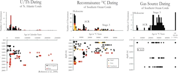
We also used a new dating technique, called the reconnaissance dating method to investigate the ecological response of deep-sea coral communities in the North Atlantic and Southern Ocean to both glaciation and rapid climate change. We find that the deep-sea coral populations of D. dianthus in both the North Atlantic and the Southern Ocean expand at times of rapid climate change. The most important factors for controlling deep-sea coral distributions are likely climatically driven changes in productivity, [O2] and [CO32-].
We take 14 deep-sea corals that we had dated to the Younger Dryas (YD) and Heinrich 1 (H1), two rapid climate change events during the last deglaciation and make U-series dates and measure clumped isotopes in them. We find that temperatures during the YD and H1 are cooler than modern and that H1 exhibits warming with depth. We place our record in the context of atmospheric and marine benthic C, C, and O records during the deglaciation to understand the role of the deep North Atlantic during the deglaciation.
We also investigated the role of climate change in the distribution of terrestrial megafauna. To help with this, we also developed a method for compound-specific
radiocarbon dating of hydroxyproline extracted from bones in the La Brea Tar Pits. We find that the radiocarbon chronologies of megafauna from several locations around the world, including the La Brea Tar Pits, exhibit an increase in abundance of megafauna during Heinrich events
TABLE OF CONTENTS
Acknowledgements ... iii
Abstract ... iv
Table of Contents ... v
List of Figures ... viii
List of Tables ... ix Chapter I: Introduction ... 1-1
Chapter II: Carbonate Clumped Isotope Thermometry of Deep-Sea Corals and Implications for Vital Effects ... 2-1
2.1 Abstract ... 2-1 2.2 Introduction ... 2-1 2.3 Methods ... 2-4 2.4 Results ... 2-5 2.4.i Internal and External Standard Errors ... 2-9 2.5 Discussion ... 2-9 2.5.i Relationship of 47 to Temperature ... 2-9 2.5.ii Vital Effect Mechanisms ... 2-15 2.5.ii.a Vital Effects in Corals ... 2-15 2.5.ii.b Diffusion ... 2-16 2.5.ii.c Mixing ... 2-18 2.5.ii.d pH ... 2-21 2.5.ii.e Other Vital Effect Models ... 2-22 2.6 Conclusions ... 2-25 2.7 References ... 2-27 Chapter III: Movement of Deep-Sea Coral Populations on Climatic Timescales ... 3-1
3.1 Abstract ... 3-1 3.2 Introduction ... 3-1 3.3 Methods and Materials ... 3-4 3.3.i Radiocarbon Method ... 3-4 3.4 Results ... 3-9 3.5 Discussion ... 3-12 3.6 References ... 3-18 Chapter IV: Evidence for the Buildup of the Thermobaric Capacitor in Deep
North Atlantic Waters during the Last Deglaciation ... 4-1 4.1 Introduction ... 4-1 4.2 Methods ... 4-5 4.2.i Radiocarbon Dating Method ... 4-5 4.2.ii U-series Method ... 4-5 4.2.iii 47 Method ... 4-6 4.3 Results ... 4-8 4.4 Discussion ... 4-22 4.5 Conclusions ... 4-29 4.6 References ... 4-31 Chapter V: Radiocarbon Chronology and the Response of Late Quaternary
Megafauna to Rapid Climate Change ... 5-1
5.1 Introduction ... 5-1 5.2 Method Development ... 5-3 5.2.i Extracting Organic Matter from Bones ... 5-3 5.2.ii Extracting Hydroxyproline from Organic Matter ... 5-6 5.3 Discussion ... 5-8 5.4 Conclusions ... 5-22 5.6 References ... 5-24
List of Figures:
Number Page 2.1 Clumped Isotope Calibration of Deep-Sea Corals ... 2-8
2.2 Internal Standard Error ... 2-10 2.3 External Standard Error ... 2-11 2.4 Offsets from Equilibrium in 47 and 18O ... 2-17 2.5 Vital Effect Mechanisms ... 2-20 3.1 Age and Depth Distribution of Deep-Sea Corals ... 3-5 3.2 Comparison of Reconnaissance Dating Method with Traditional Method ... 3-7 3.3 Radiocarbon Standard Data ... 3-7 3.4 Comparison of Different Radiocarbon Dating Methods ... 3-8 3.5 YD, ACR, and H1 Profiles ... 3-10 3.6 Late Holocene Distribution ... 3-11 3.7 Holocene Distribution ... 3-15 4.1 Ice Core and Marine Reconstructions of Climate Evolution ... 4-2 4.2 Clumped Isotope Cleaning Study ... 4-7 4.3 YD and H1 Temperature and C Profile ... 4-9 4.4 Vital Effects in Deep-Sea Corals ... 4-21 4.5 Potential Temperature and Salinity for YD and H1 ... 4-23 4.6 Benthic C and 13C over the Deglaciation ... 4-25 5.1 %C and 13C Results of Cleaning Study ... 5-5 5.2 C Results of Cleaning Study ... 5-7 5.3 HPLC Traces of Amino Acid Standard and La Brea ... 5-9 5.4 Sample Peak Area Calibration ... 5-10 5.5 Hydroxyproline 14C ... 5-11 5.6 La Brea Radiocarbon Dates and ECDF ... 5-12 5.7 Radiocarbon Chronologies of Megafauna Distributions ... 5-16 5.8 Comparison of Rapid Climate Change Events to Background (by Area) .. 5-17 5.9 Comparison of Rapid Climate Change Events to Background (by Time) .. 5-18
List of Tables
2.1 Modern Deep-Sea Coral C, O and 47 values ... 2-7 3.1 Radiocarbon and Calendar Ages for North Atlantic Corals ... 3-22 3.2 Radiocarbon and Calendar Ages for Tasmanian Corals ... 3-24 3.3 Statistical Results Comparing Different Populations ... 3-28 3.4 Radiocarbon and U-Series Dates for ACR ... 3-29 4.1 ames and Depths of Corals Analyzed ... 4-10 4.2 Clumped Isotope Measurements of Corals ... 4-10 4.3 Individual Clumped Isotope Measurements of Corals and Standards ... 4-11 4.4 eated Gas Measurements ... 4-17 4.5 Corals Displaying VIE in Clumped Isotopes ... 4-19 4.6 14C Age of Corals ... 4-20 4.7 U-Th of Corals ... 4-20
Chapter 1 Introduction
The ocean is considered a key parameter during glacial-interglacial transitions and rapid climate change events, as it is one of the largest reservoirs of CO2 and heat in the atmosphere-climate system. The most common and successful approach to
reconstructing past ocean conditions take advantage of isotopic and elemental substitution into foraminiferal CaCO3 in sediment cores to determine a variety of parameters, including temperature, nutrient ratios, and carbon systematics. Here we develop the use of deep-sea corals as a paleoclimate archive.
Deep-sea corals are a relatively new archive in paleoceanography. Their banded skeletons can be used to generate 100 year high-resolution records without bioturbation.
They also have a high concentration of uranium, allowing for accurate independent calendar ages using U–Th systematics. These characteristics make them particularly suited for
studying the deep ocean, especially on timescales relevant to rapid climate change. In this work we are interested in understanding the capacity of the ocean to influence rapid climate change. We approach this issue by monitoring and developing new tools to determine deep ocean chemistry recorded in the deep-sea corals.
In Chapter 2 , we calibrate the carbonate clumped isotope thermometer in modern deep-sea corals. We examined 11 specimens of three species of deep-sea corals and one species of a surface coral spanning a total range in growth temperature of 2–25oC. Internal standard errors for individual measurements ranged from 0.005‰ to 0.011‰ (average:
0.0074‰) which corresponds to 1–2oC. External standard errors for replicate measurements of ∆47 in corals ranged from 0.002‰ to 0.014‰ (average: 0.0072‰) which corresponds to 0.4–2.8oC. This result indicates that deep sea corals can be used for paleothermometry, with precisions as good as 0.4oC. We also observe no vital effects in ∆47 for samples that display large vital effects in δ18O and δ13C. We explore several reasons for why the clumped isotope
composition of deep-sea corals exhibit no evidence of a vital effect and conclude that pH effects could explain the observed variations in ∆47 and δ18O.
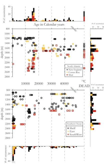
In chapter 3, we use a new dating technique, called the reconnaissance dating method to investigate the ecological response of deep-sea coral communities in the North Atlantic and Southern Ocean to both glaciation and rapid climate change. We find that the deep- sea coral populations of D. dianthus in both the North Atlantic and the Southern Ocean expand at times of rapid climate change. However, during the more stable Last Glacial Maximum the coral population globally retreats to a more restricted depth range. Holocene populations show regional patterns that provide some insight into what causes these
dramatic changes in population structure. The most important factors are likely responses to climatically driven changes in productivity, [O2] and [CO32-].
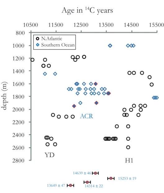
In chapter 4, we take advantage of the results of the previous two chapters. We analyze 14 deep-sea corals that we had dated to the Younger Dryas (YD) and Heinrich 1 (H1), using the reconnaissance dating technique and make high-precision radiocarbon dates, U-series dates and clumped isotope measurements. We find that temperatures during the YD and H1 are cooler than modern and that H1 exhibits warming with depth. This warming at depth supports the “Thermobaric Capacitor” hypothesis for causing deep ocean mixing. We place our record in the context of atmospheric and marine benthic ∆14C, δ13C and δ18O records during the deglaciation to understand the role of the deep North Atlantic during the deglaciation.
In chapter 5, we investigate the effects of rapid climate change on the terrestrial biosphere, particularly the distribution of terrestrial megafauna. Current hypotheses for the extinction of megafauna focus on human interactions or environmental change. Most of the climate change hypotheses emphasize either changes in habitat or the fast rate of climate change. To further explore the relationship of megafauna to rapid climate change, we examine the abundance of megafauna in the La Brea Tar Pits during the YD and H1.
The La Brea Tar Pits are an exceptionally well preserved archive that has trapped
over three million fossil skeletons including 3400 large mammals. The deposits are a series of open asphalt seeps that have acted as animal traps for at least the past 50,000 years.
Previous studies have been limited by weak chronological control, as stratigraphic position is known to be an unreliable indicator of relative age within the asphalt deposits and the asphalt itself has been a large source of carbon contamination. To help with this, we have developed an HPLC method for compound-specific radiocarbon dating of hydroxyproline extracted from bones in the La Brea Tar Pits. We find that in La Brea and other locations around the world, the megafauna abundance actually increases. Therefore megafauna extinctions were either primarily caused by humans, a climatic variable that did not adversely affect megafauna during rapid climate change events, or some combination of the two.
Chapter 2
Carbonate Clumped Isotope Thermometry of Deep-Sea Corals and Im- plications for Vital Effects
2. ABSTRACT
We examined specimens of three species of deep-sea corals and one species of a surface coral spanning a total range in growth temperature of 2 ̶ 25oC. Analytical precision for individual measurements ranged from 0.005 to 0.011‰ (average: 0.0074‰) which corresponds to ~ to 2oC. Analytical precision for replicate measurements of D47 in corals ranged from 0.002 to 0.014‰ (average: 0.0072‰) which corresponds to 0.4 to 2.8oC. We find that skeletal carbon- ate from deep-sea corals shows the same relationship of Δ47 (the measure of 3C-18O ordering) to temperature as does inorganic calcite. In contrast, the δ18O values of these carbonates (measured simultaneously with Δ47 for every sample) differ markedly from equilibrium with seawater; i.e., these samples exhibit pronounced ‘vital effects’ in their bulk isotopic compositions. We explore several reasons why the clumped isotope compositions of deep-sea coral skeletons exhibit no evidence of a vital effect despite having large conventional isotopic vital effects.
2.2 INTRODUCTION
Oxygen isotope measurements of biogenic marine carbonates are a long established and important tool for determining past ocean temperatures (Epstein et al., 1953; McCrea, 1950;
Urey, 1947). In the decades following its initial development, the δ18O thermometer was applied to planktonic foraminifera to reconstruct ocean temperature shifts on glacial/interglacial time scales (Emiliani, 1955). However it was later recognized that the planktonic record reconstruct- ed from foraminifera δ18O reflects a combination of the temperature from which the carbonate grew, and global changes in ice volume (Shackleton, 1967).
Deconvolving these two effects on the marine-carbonate oxygen isotope record remains a central problem in paleoclimatology. Chappell and Shackleton (1986) addressed this problem by examining dated coral terraces and benthic δ18O records. Previously, the benthic δ18O re- cords had been interpreted assuming a constant temperature in the abyssal ocean. However, the resulting ice volume estimates derived from benthic δ18O records could not be reconciled with ice volume records derived from the altitudes of dated coral terraces. Chappell and Shackleton (1986) made a detailed comparison of a coral terrace record in the Huon Peninsula with a benthic δ18O record from the Pacific Ocean and concluded that during the last interglaciation, abyssal temperatures changed only during the transition from Marine Isotope Stage (MIS) 5e to 5d, and during the last glacial termination.
Subsequent efforts have reconstructed the δ18O of the water of the deep ocean during the Last Glacial Maximum based on isotopic analyses of marine pore fluids (Schrag and DePaolo, 1993). Cutler et al. (2003) reconstructed a sea level curve based on fossilized surface corals from the Huon Peninsula and Barbados and combined this new sea level curve with the δ18O of the water of the deep ocean reconstruction determined from pore fluids (Adkins et al., 2002).
This work established that deep-sea temperatures have warmed by 4oC in the Atlantic and 2oC in the Pacific since the Last Glacial Maximum. In all of these studies, independent estimates of the change in sea level or of the δ18O of the water of the deep ocean were necessary to extract deep ocean temperatures from benthic δ18O data.
Carbonate clumped isotope thermometry is a new temperature proxy based on the order- ing of 3C and 18O atoms into bonds with each other in the same carbonate molecule. The propor- tion of 3C and 18O atoms that form bonds with each other in a carbonate mineral has an inverse relationship with growth temperature. This isotopic ‘clumping’ phenomenon exists due to a
thermodynamically controlled homogeneous isotope exchange equilibrium in the carbonate min- eral (or, perhaps, in the dissolved carbonate-ion population from which the mineral grows). This exchange reaction is independent of the δ18O of water and δ3C of DIC from which the carbonate grew; therefore it can be applied to settings where these quantities are not known (Eiler et al., 2003; Eiler and Schauble, 2004; Ghosh et al., 2006).
Here we calibrate carbonate clumped isotope thermometry in modern deep-sea corals.
Deep-sea corals are a relatively new archive in paleoceanography. Their banded skeletons can be used to generate ~ 00-year high-resolution records without bioturbation. They also have a high concentration of uranium, allowing for accurate independent calendar ages using U-Th system- atics. A thermometer in deep-sea corals could address the phasing of the offset between North- ern and Southern Hemisphere in rapid climate events. The Greenland and Antarctic ice cores both show that temperature and CO2 are tightly coupled over the last several glacial interglacial events. However, the synchronization of the ice cores from the two regions using atmospheric methane concentration trapped in the ice layers revealed that Antarctica warms several thousand years before the abrupt warmings in the Northern Hemisphere (Blunier and Brook, 2001). The deep ocean is a massive heat and carbon reservoir with an appropriate time constant that could be used to explain the several thousand year offset between the hemispheres. A temperature record of the deep ocean that spans the time period of these rapid climate events would help explain the role of the deep ocean in rapid climate change events.
Deep-sea corals are also an important resource to study vital effects because they grow without photosymbionts and grow in a relatively homogeneous environment with minimal varia- tions in temperature and the composition of co-existing water. Therefore, offsets from equilib- rium that we observe in any chemical proxies can be attributed to biological processes associated
with calcification. Previous work in surface and deep-sea corals has found evidence of isotopic disequilibrium in δ3C and δ18O (Adkins et al., 2003; Emiliani et al., 1978; McConnaughey, 1989; Weber and Woodhead, 1970; Weber, 1973). McConnaughey attributes these offsets in surface corals to kinetic and metabolic effects. However light-induced metabolic effects cannot be invoked to explain offsets in deep-sea corals because they do not have any photosymbionts.
Radiocarbon dating of modern corals and their surrounding dissolved inorganic carbon (DIC) also indicate that the skeletal material of deep-sea coral is drawn almost entirely from the ambi- ent inorganic carbon pool and not from respired CO2 (Adkins et al., 2003). Due to the correla- tion between growth banding and stable isotopes within individual corals, Adkins et al. (2003) proposed that vital effects in deep-sea corals involve a thermodynamic response to a biologically induced pH gradient in the calcifying region. Watson (2004) proposed a surface entrapment model in which growth rate, diffusivity, and the surface layer thickness all control crystal com- position. In this model, the trace element or isotope composition of the crystal is determined by the concentration of that element in the near-surface region and the outcome of the competition between crystal growth and ion migration in the near-surface region.
More recently, Ghosh et al. (2006) found evidence of an anomalous enrichment in Δ47 values in winter growth bands in a Porites sample from the Red Sea, suggesting that surface cor- als may have a vital effect in this parameter. Here we look at a variety of deep-sea corals grown from different locations, and analyze their Δ47 values to develop a modern calibration for carbon- ate clumped isotope thermometry and to investigate the mechanisms of vital effects.
2.3 METHODS
Samples examined in this study were obtained from the Smithsonian collection (Na- tional Museum of Natural History). We focused on Desmophyllum sp., Caryophyllia sp., and
Ennalopsammia sp. collected from a variety of locations and depths. One Porities sp. coral from the Red Sea was also analyzed. Isotopic measurements were made on pieces from the septal region of the coral that were cut using a dremel tool. For each clumped isotope measurement, eight to fifteen mg from each coral was analyzed. The outsides of the coral were scraped with a Dremel tool to remove any organic crusts. The sample was then digested in 03% anyhydrous phosphoric acid at 25oC overnight. The product CO2 was extracted and purified using methods described previously (Ghosh et al., 2006).
Evolved CO2 was analyzed in a dual inlet Finnigan MAT-253 mass spectrometer with the simultaneous collection of ion beams corresponding to masses 44-49 to obtain Δ47, Δ48, Δ49, δ3C and δ18O values. The mass 47 beam is composed of 17O3C17O, 17O2C18O and predomi- nantly 18O3C16O and we define R47 as the abundance of mass 47 isotopologues divided by the mass 44 isotopologue. (R47=[17O3C17O+ 17O2C18O+18O3C16O]/[16O2C16O].) Δ47 is reported relative to a stochastic distribution of isotopologues for the same bulk isotopic composition.
(Δ47=(((R47measured/R47stochastic)-1)- ((R46measured/R46stochastic)-1)- ((R45measured/R45stochastic)-1))*1000. ) Mass- es 48 and 49 were monitored to detect any hydrocarbon contamination. Measurements of each gas consisted of 8 ̶ 26 acquisitions, each of which involved 10 cycles of sample-standard com- parison with an ion integration time of 20 s per cycle. Internal standard errors of this population of acquisition to acquisition for Δ47 ranged from 0.005 ̶ 0.01‰, (1 ̶ 2oC) while external standard error ranged from 0.002 ̶ 0.014‰ (0.4 ̶ 2.7oC). The internal standard error for d13C ranged from 0.5 ̶ 1 ppm and the internal standard error for d18O ranged from 1 ̶ 3 ppm.
2.4 RESULTS
Table 2.1 summarizes results of isotopic analyses of all coral samples investigated in this study. A 0.16‰ range in Δ47 was observed among coral samples having an estimated range in
growth temperature of 2 ̶ 25oC (Table 2.1; Fig. 2.1). Table 2.1 also reports the δ18OPDB values of corals analyzed in this study, along with growth temperatures, and the δ18O values of the water from which the corals grew. The δ18O of the water from which the coral grew was reconstructed through a combination of the LEVITUS salinity database (http://ingrid.ldeo.columbia.edu/
SOURCES/.LEVITUS94/.ANNUAL/.sal/) and the NASA δ18O of seawater database (http://data.
giss.nasa.gov/cgi-bin/o18data/geto18.cgi). The LEVITUS database is more finely gridded for salinity than the NASA database. So we determined the relationship between δ18O of the seawa- ter and salinity near the sample site and used the salinity as determined by LEVITUS to calcu- late the δ18O of the seawater from the δ18O of the seawater vs. salinity relationship. The total error on the calculated δ18Osw calculated ranged from 0.1 ̶ 0.2‰.
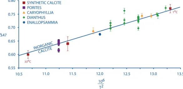
Figure 1 plots the Δ47 values of deep-sea corals vs. their nominal growth temperatures.
The Porites surface coral BIR- has significant error bars in the temperature axis, unlike the deep-sea coral samples (where growth temperatures do not vary significantly seasonally), be- cause it was collected in the Red Sea and sea surface temperatures range from 22 ̶ 28oC through the year (Ghosh et al., 2006). Ghosh et al. (2006) found vital effects in the winter band of BIR-1.
Our analyses are of one annual band that was crushed and homogenized, and we do not observe any offsets from equilibrium. This inconsistency could be because winter bands do not contrib- ute a significant portion of the annual cycle.
The relationship of Δ47 to temperature is similar to that of inorganic precipitates. In a plot of Δ47 vs. /T2 the two species of solitary corals, Desmophyllum (slope: 0.0495 ± 0.012; inter- cept: 0.1052 ± 0.1557) and Caryophyllia (slope: 0.05545 ± 0.008; intercept: 0.0302 ± 0.1116) are indistinguishable in slope and intercept from the inorganic calibration line (slope: 0.0597
± 0.004; intercept:-0.03112 ± 0.0475). Note, however, that these equations are not suitable for
Table 1
Name Genus Ƥ13C Ƥ18Omineral
Growth Temperature
(oC) ƅ47 error in ƅ47 Ƥ18Ow
47413 Desmophyllum -5.009 0.723 7.9 0.733 0.007 -0.439
47413 Desmophyllum -6.274 0.343 7.9 0.736 0.006 -0.439
47413 Desmophyllum -4.877 0.686 7.9 0.732 0.009 -0.439
47413 Desmophyllum -4.720 0.764 7.9 0.736 0.008 -0.439
47413 Desmophyllum -6.285 -0.006 7.9 0.722 0.005 -0.439
47413 Desmophyllum -4.544 0.833 7.9 0.726 0.007 -0.439
47413 Desmophyllum -6.286 0.032 7.9 0.697 0.006 -0.439
80404 Desmophyllum -1.230 1.535 13.1 0.707 0.009 0.25
80404 Desmophyllum -1.826 1.764 13.1 0.695 0.008 0.25
80404 Desmophyllum -1.185 1.611 13.1 0.717 0.010 0.25
47407 Desmophyllum -5.640 0.768 4.2 0.749 0.006 -0.047
48738 Desmophyllum -1.478 2.987 9.8 0.762 0.010 0.624
48738 Desmophyllum -1.567 2.968 9.8 0.715 0.005 0.624
48738 Desmophyllum -4.897 1.537 9.8 0.727 0.008 0.624
47409 Desmophyllum -3.640 1.171 2.3 0.772 0.008 -0.088
62308 Desmophyllum -4.725 1.147 3.7 0.744 0.010 0.5
77019 Ennallapsammia -0.212 3.670 14.3 0.675 0.004 0.95
47531 Ennallapsammia -1.603 0.982 7.5 0.738 0.009 -0.14
49020 Caryophyllia 0.708 1.548 17.4 0.688 0.011 0.907
45923 Caryophyllia 0.289 3.139 4.6 0.744 0.008 0.68
1010252 Caryophyllia -0.115 2.818 6.1 0.744 0.008 0.222
BIR-1 Porites -1.092 -3.720 25.2 0.650 0.006 1.91
BIR-2 Porites -1.183 -3.670 25.2 0.639 0.006 1.91
BIR-3 Porites -1.186 -3.659 25.2 0.648 0.005 1.91
BIR-4 Porites -1.195 -3.664 25.2 0.615 0.007 1.91
10.5 11.0 11.5 12.0 12.5 13.0 13.5 0.55
SYNTHETIC CALCITE PORITES
CARYOPHYLLIA DIANTHUS ENALLOPSAMMIA
INORGANIC CALCITE
106 T2
∆47
0.60 0.80
0.65 0.70
0.75 1oC
33oC
Figure 2.1: Clumped isotope calibratino of deep-sea corals and Porites, a surface coral. The dashed line is the inorganic calibration line as determined by measuring CO2 produced from synthetic carbonates grown in the laboratory at known and controlled temperatures (Ghosh et al.
2006).
extrapolation beyond the range of observations (0 ̶ 50oC).
2.4.i Internal and External Standard Errors
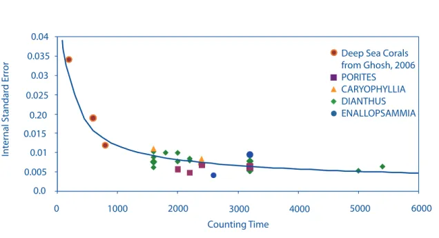
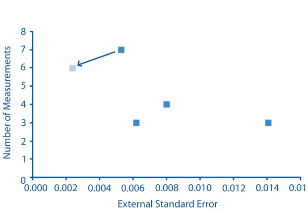
The average standard error for our Δ47 measurements are in agreement with the shot noise limit predicted for the analyses (Fig 2.2). Samples that were run for several hours have the low- est standard error, on the order of 0.005‰, which corresponds to a 1oC temperature change for low temperatures on the Ghosh et al. (2006) temperature scale. Several of the corals examined in this study were analyzed multiple times each, permitting us to estimate the external reproduc- ibility for individual measurements of a given sample. This external standard error (i.e., the standard error of the average of multiple extractions) ranges from 0.005 to 0.014‰ (1 ̶ 2.8oC), and decreases with the number of measurements (Fig 2.3). If one extraction of sample 47413 (a measurement we suspect was compromised by exchange of water) is excluded from these sta- tistical calculations, the external standard error ranges from 0.002 ̶ 0.014‰ (0.4 ̶ 2.8oC). This external standard error is still larger than the expected shot noise errors for the same samples (~
0.0025 ̶ 0.0040‰).. The difference in external standard error from expected shot noise limits may be due to sample heterogeneity, unaccounted for analytical fractionations, or contaminants in the sample.
The reproducibility we document has implications for future analyses of deep-sea corals.
If sample size is limited, the best precision attainable is 0.005‰ (±1oC). However if sample size is not the limiting factor, the coral is homogenous, and not contaminated or otherwise analyti- cally fractionated, precision is demonstrably as good as 0.002‰ (±0.4oC).
2.5. DISCUSSION
2.5.i Relationship of Δ47 to Temperature
For two of the solitary coral genera analyzed in this study, each exhibit slopes and in-
Deep Sea Corals from Ghosh, 2006 PORITES
CARYOPHYLLIA DIANTHUS ENALLOPSAMMIA
0 1000 2000 3000 4000 5000 6000
0.0 0.005 0.01 0.015 0.025
Counting Time
Internal Standard Error
0.20 0.03 0.035 0.04
Figure 2.2: Internal standard error of our measurements with counting time. The dark line is the shot noise calculation. The error in our measurements is dominated by shot noise errors and decreases with increasing counting time.
Figure 2.3: A figure of the external standard error of our measurements. Multiple replicates de- creases the standard error of our measurements. The arrow indicates how coral 47413 changes if one extraction (suspected of having exchanged with water) is removed.
0.000 0.002 0.004 0.006 0.008 0.010 0.012 0.014 0.016 0
1 2 5 3 4 6 7 8
External Standard Error
Number of M easur emen ts
tercepts in a plot of Δ47 vs. /T2 that are within error of the inorganic calibration line (Fig 2.1).
Since the publication of the Ghosh et al. (2006) calibration, several more measurements have been made of inorganic calcite, foraminifera, mollusks, and soil carbonates having independently known growth temperatures. Most of these previous measurements are indistinguishable from the inorganic calibration line (Came et al., 2007; Daeron, 2007; Tripati, 2007). There have how- ever been nonequilibrium results obtained for speleothems and some synthetic carbonates (Affek et al., 2008; Guo, 2009). A recently published calibration for inorganic synthetic calcite (Dennis and Schrag, 2010) also disagrees with the Ghosh et al. (2006) result at low temperatures (< ~ 15˚C). The source of this discrepancy is unclear; it could reflect some combination of analytical artifacts (including intralaboratory calibration discrepancies) and/or kinetic isotope effects in car- bonate synthesis reactions in either or both studies. We simply note here that this study presents data for 15 samples analyzed in this low temperature range, and they follow a temperature-de- pendence closely similar to that proposed by Ghosh et al. (2006), but steeper than that presented by Dennis and Schrag (2010). We suggest two straightforward explanations for this result: either the Ghosh et al. (2006) data reflect a kinetic isotope effect at low temperature that is mimicked by a vital effect in deep-sea corals (and, similarly, other classes of organisms previously observed to conform to the Ghosh et al. (2006) trend), yet independent of the vital effect on d18O and d13C in those corals (see below); or the Dennis and Schrag (2010), calibration is influenced by a ki- netic isotope effect in low-temperature experiments. In the absence of any additional constraints, the second of these seems to us to be the more plausible explanation, and we will presume this for the rest of this discussion. But, we emphasize that inorganic calibrations will likely remain a subject of ongoing research and this interpretation should be revisited as new data come to light.
Three individual analyses made as part of this study are inconsistent with the inorganic
calcite calibration trend (i.e., differ from it by more than 2 sigma external error). Two of the outliers are an extraction from each of the samples 47413 and 48738. These outliers were extrac- tions from corals that have been analyzed several times, and in both cases all other extractions from that sample exhibited no offset in Δ47 from the inorganic calibration line. Sample 47413 is unusual because, although the outlier was free of recognized contaminants, it did have a higher Δ47 and lower δ18O than all the other replicates of that sample. This combination indicates that it could have exchanged with water (Pasadena tap water: 25oC, δ18O =-8‰) at some point during sample processing. Sample 48738 has an orange organic crust coating it, implying that perhaps it is not modern or that the organic coating was not completely removed prior to sample process- ing and affected the measurement. In any event, these two measurements are irreproducible exceptions to the otherwise straightforward trend produced by all other analyses, and thus we do not believe they indicate any systematic discrepancy between corals and inorganic calcite in Δ47 systematics. The third outlier is 77019, an Enallopsammia from 30oN, 76oW at 494 m of water depth in the core of the Gulf Stream, a region known for seasonal and interannual variations in salinity. This coral is also peculiarly enriched in d18O indicating possible uncertainties in the d18Ow reconstructed at this site.
The accuracy of deep-sea coral temperature estimates based on the calibration in Figure 2.1 will depend on uncertainties in both the Δ47 of the sample and uncertainties in the calibration line, whereas the precision of sample-to sample differences will depend only on the Δ47 measure- ments of samples. If one considers all previous measurements of published and unpublished inorganic and biogenic calibration materials (egg shells, teeth, otoliths, mollusks, brachiopods, corals and foraminifera; we exclude here the recent inorganic data of Dennis and Schrag (2010), discussed above) to be part of a single trend (i.e., because trends defined by each material are
statistically indistinguishable), then they make up a calibration line of slope in D47 vs. /T2 space of 0.0548+/-0.0019 and intercept of -0.0303+/-0.0221. The standard error of the calibration is 0.0018‰. If one excludes otoliths, which differ most from the other trends (perhaps due to a small vital effect, or due to inaccuracies in estimated body temperatures, or some other fac- tor) and planktic foraminifera (where the variation in temperature with water depth and season is large and therefore a mean hard to estimate with confidence), the calibration line has a slope and intercept of 0.0562 +/- 0.0020 and 0.0167 +/- 0.0226. The standard error in the calibration is then 0.0019‰. The formal errors in slope and intercept of the overall calibration are trivially small; though one should not extrapolate the fitted trend outside of its range in calibration tem- peratures (particularly at higher temperatures, where the slope flattens considerably; (Dennis and Schrag 2010, Eiler, 2009). Thus, barring some unrecognized systematic error in all of the cali- bration data sets, the accuracy of temperature estimates of samples is dominated by error in the Δ47 measurement of the sample, which is generally dominated by shot noise error. The shot noise error for Δ47 analyses under normal analytical conditions generally levels off (ceases to improve with increased counting time) at ~ 0.005‰ (or ~ 1oC) after 4500 seconds or ~ 20 acquisitions.
Current analytical methods require 11 mg of CaCO3 for 4500 seconds (i.e., to achieve 0.005‰
precision). If large amounts of homogeneous sample are available, precision could be improved further by combining data from multiple measurements of 11 mg sample aliquots. Sub degree precisions should be possible in this case. For example, if 11 mg of coral analyzed for 4500+
seconds resulted in a measurement of 2o C with a standard error of 0.005‰, or 1o C, then six mg measurements of the same homogeneous coral could result in a precision as low as 0.002‰
or 0.4oC (plus the small error in the accuracy of the calibration). Or, if three replicate measure- ments were made for the top of a deep-sea coral and six of the bottom of the same deep-sea coral
(i.e., if one were searching for evidence of temperature change over the course of its growth), the error in the temperature estimate at the top would be ± 0.4oC, the error in the temperature at the bottom would be ± 0.7oC, and the temperature difference (ΔT=top temperature-bottom tempera- ture) would have an error of ± 0.8 (because the two errors would be added in quadrature).
2.5.ii Vital Effects Mechanisms 2.5.ii.a Vital Effects in Corals
Use of deep-sea corals (and other biogenic carbonates) as a paleoceanographic archive is complicated by a set of biological processes commonly referred to as vital effects. Vital effects have been observed in aragonitic corals as offsets from equilibrium in stable isotope and metal/
calcium ratios for a given temperature and other equilibrium conditions. Vital effects in corals and other organisms have also been noted to be dependent on growth rate, kinetics, pH, light and to the presence or absences of photosymbionts (Cohen et al., 2002; McConnaughey, 1989; Reyn- aud et al., 2007; Rollion-Bard et al., 2003; Weber and Woodhead, 1970).
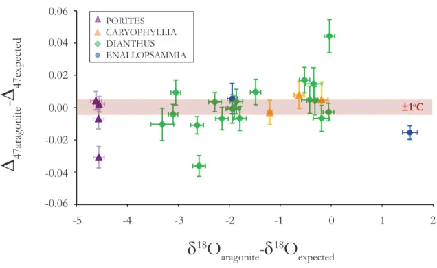
The range of vital effects in conventional, or ‘bulk’ stable isotope compositions seen in deep-sea corals is 7‰ in δ18O and 12‰ in δ3C. In contrast, Δ47 values do not appear to exhibit any vital effects (i.e., they remain indistinguishable from the inorganic calibration across the full studied temperature range). The analytical method used to determine Δ47 values simultane- ously generates δ3C and δ18O values for the sample; therefore, it is possible for us to evaluate the extent to which each analyzed sample expressed ‘vital effects’ in their O and C isotope composi- tions. A plot of Δ47measured- Δ47expected vs δ18Omeasured- δ18Oexpected does not show any correlated trends, and there are no systematic deviations in Δ47measured from Δ47expected even when there are clearly offsets in δ18O (Fig 2.4). While our study was not designed to examine the mechanisms of vital effects, our results offer new constraints on this problem.
The following sections compare our results with the predictions one would make based on various previously proposed vital effect mechanisms.
2.5.ii.b Diffusion
Diffusion of CO2 through a lipid bilayer or of different carbonate species across a fora- minifer shell has been proposed as a part of different vital effect models (Adkins et al., 2003;
Zeebe et al., 1999, Erez, 2003). While we do not have a first principle understanding of how this type of diffusion might affect the ∆47 value, we can use other types of well-known diffusion to inform this discussion. The kinetic theory of gases predicts that a gas that is diffused through a small aperture (‘Knudsen diffusion’) will be depleted in heavy isotopes relative to the residual gas it leaves behind. This behavior is described by the equation Rjdiffused = Rjresidue(Mi/Mj)0.5 where Rj is the ratio of the concentration of isotopologue j to i and M is the mass.
Knudsen diffusion predicts that for a CO2 population that has undergone diffusive frac- tionation, the diffused gas will be 11.2‰ lower in δ3C, and 22.2‰ lower in δ18O, but only 0.5‰
higher in Δ47. This seemingly counterintuitive behavior is due to the nonlinear dependence of the stochastic abundances of mass-47 CO2 isotopologues on the bulk isotopic composition (Eiler and Schauble, 2004). For natural isotopic compositions, the stochastic abundance increases more for an incremental change in δ3C or δ18O than does the vector that describes diffusive fractionation in δ3C, δ18O and Δ47 space. Therefore, a diffused population of gas would be more depleted in δ3C and δ18O but higher than expected in Δ47.
Similarly, gas phase inter diffusion where gas A diffuses through gas B is described by the relation Da/Da’={(Ma+Mb)/(MaMb)x(M’aMb)/(M’a+Mb)0.5}, where Ma is the mass of the dif- fusing molecule, Mb is the mass of the gas through which gas A is diffusing and the primes indicate the presence of a heavy isotope. The gas phase diffusion of CO2 through air generates
PORITES CARYOPHYLLIA DIANTHUS ENALLOPSAMMIA
∆
47aragonite- ∆
47expectedδ
18O
aragonite-δ
18O
expected2 1
0 -1
-2 -3
-4 -5
0.00
-0.06 -0.04 -0.02 0.02 0.04 0.06
±1oC
Figure 2.4: Offsets from equilibrium in D47 and d18O. The biggest offsets in D47 are from corals with multiple extractions and every other extraction from those corals have no offset in D47 .
fractionations of -4.4‰ for δ3C, -8.7‰ for δ18O and +0.3‰ for Δ47. The enrichment of Δ47 in the diffused phase is again due to the relatively strong dependence of the stochastic abundance of mass-47 CO2 on the bulk isotopic composition.
Isotopic fractionations caused by diffusion of molecules through a liquid medium are generally smaller than those associated with gas-phase diffusion. For instance, the ratio of dif- fusion coefficients of 2CO2 and 3CO2 in water is 1.0007 (O’Leary, 1984), whereas the gas phase interdiffusion equation, taking the medium to be H2O predicts a fractionation factor of .0032.
However, these condensed phase diffusive fractionations are generally described through a power-law relationship (i.e., the fractionation factor scales as the ratio of masses to some power, generally less than 0.5) (Bourg and Sposito, 2008). In this case, the mass dependence of the diffusive fractionation remains the same as for Knudsen diffusion, and the slope followed in a plot of ∆47 vs. d18O or d3C will remain the same. If so, then liquid phase diffusion of CO2 should result in fractionations of -0.7‰ for δ13C (i.e., the experimental constraint), -1.6‰ for δ18O and +0.036‰ for Δ47. On Figure 2.5 we have also indicated what 10% of the Knudsen and gas phase interdiffusion vector are to emphasize the difference between the scale of the different vectors.
If deep-sea coral growth involved nonequilibrium isotopic fractionations that were dominated by diffusion across a lipid bilayer or in an aqueous medium, then a plot of Δ47 vs. δ18O might have the same slope as the vectors that describe the types of diffusion discussed above. However the data is inconsistent with any of these predicted slopes (Fig 2.5). In addition, all of the diffusive processes predict δ3C variations smaller than δ18O variations, which is opposite to what is seen in deep-sea corals.
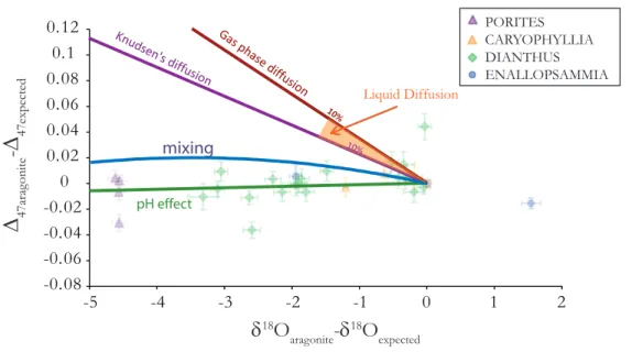
2.5.ii.c Mixing
The stochastic distribution that defines the reference frame for reporting Δ47 values has a
subtle saddle-shape curvature in a 3-dimensional plot of δ3C vs. δ18O vs. R47. Therefore, con- servative mixing of two CO2 populations with the same Δ47 but different δ3C and δ18O leads to a mixed population having a different Δ47 value than the weighted sum of the Δ47 values of the end members (Eiler and Schauble, 2004).
Deep-sea corals have a large variation in δ3C and δ18O and could possibly produce ∆47 signals solely from this mixing effect. The range of variations seen in a single coral can be as large as 12‰ in δ3C and 7‰ in δ18O (Adkins et al., 2003). Two example end members seen in δ3C and δ18O are δ3C=-10‰ and δ18O=-2‰, and δ3C=2‰ and δ18O=5‰. If the stable isotopic variation in a deep-sea coral reflects variation in the DIC pool that the coral was using for cal- cification, we can calculate what magnitude of Δ47 offset would result from mixing between the isotopic end members of the DIC pool. However, the carbonate species of interest for calcifica- tion is not CO2 (and its ∆47 value) but CO3 and its corresponding 3C-18O clumped isotopologue.
The relevant isotope exchange reaction for CO3 species is:
2C18O16O22-+3C16O32-< -- > 3C18O16O22- + 2C16O32-.
So, we calculated the mixing effect on ∆63 (i.e., enrichment in mass-63 carbonate ion iso- topologues, analogous to the Δ47 values of CO2) and then converted this to a ∆47 value that would be measured in a coral skeleton. If both the high- and low- δ3C and δ18O share a common “Δ63” value then we predict the amplitude of this mixing effect is as large as 0.02‰ for the case of 50%
of each end member (which would generate the largest Δ63 offset, and still a relatively large offset in δ18O). Because phosphoric acid is believed to produce CO2 having a Δ47 value that is offset by a constant amount from the Δ63 value of reactant carbonate (for a fixed temperature of reaction) this 0.02‰ enrichment due to mixing should be directly inherited by analyzed CO2 (Guo et al., 2009). It is clear that this mixing model is inconsistent with the data, as there is no curvature to
-0.08 -0.06 -0.04 -0.02 0 0.02 0.04 0.06 0.08 0.1 0.12
-5 -4 -3 -2 -1 0 1 2
mixing
Liquid Diffusion
pH effect
∆ 47aragonite-∆ 47expected
δ18Oaragonite-δ18Oexpected
PORITES CARYOPHYLLIA DIANTHUS ENALLOPSAMMIA
Figure 2.5: Vectors describing how various processes effect D47 and d18O. Diffusive and mixing processes cannot explain the coupled variation in D47 and d18O; however pH effects can.
the Δ47 vs. δ18O trend unlike the mixing model (Figure 2.5). However, it is possible that mixing accompanied by re-equilibration would generate a horizontal line, and thus be more consistent with the data. Further experiments are needed to determine the rate that carbonate precipitating from DIC incorporates the different clumped carbonate species in DIC and whether mixing and subsequent re-equilibration would be recorded in the precipitating carbonates.
2.5.ii.d. pH
It has been demonstrated for inorganically precipitated carbonates that higher pH values (and thus higher CO32- proportions in DIC) result in isotopically lower δ18O values (McCrea, 1950; Usdowski et al., 1991). This observation has been explained by the pH dependent specia- tion of the DIC pool from which carbonate precipitates and the different fractionation factors between water and these DIC species. At seawater like pHs HCO3- dominates and at high pHs CO32- dominates the DIC. McCrea (1950) and Usdowski et al. (1991) demonstrated that if cal- cium carbonate is quantitatively precipitated from a bicarbonate-carbonate solution, the oxygen isotopic composition of the solid reflects the weighted average of all the fractionation factors with respect to water for all the carbonate species. Zeebe (1999) exploited this observation to explain the variation seen in the inorganic carbonate data in Kim and O’Neil (1991) and existing stable oxygen isotope ratios of foraminiferal calcite.
It would be helpful to understand how the clumped isotope composition of the DIC varied with pH. Guo et al., (2008) theoretically estimated the Δ63 values of dissolved carbonate species in water; at 300K, CO32- has a predicted value of 0.403‰, whereas HCO3- has a value of 0.421‰. While the absolute values of these calculated Δ63 estimates vary with the parameter- ization of the computational model, the offset between CO32- and HCO3- remains constant at ~ 0.018‰, and thus is likely a robust feature of the calculation (Guo et al., 2008). The equivalent
difference in δ18O at 19oC is 34.3‰ for HCO3- and 18.4‰ for CO32- (Zeebe, 1999).
Given Zeebe’s model of precipitation and Guo et al.’s (2008) calculated differences in Δ63 be- tween HCO3- and CO32-, we estimate the pH dependence of Δ63 of carbonate (which we take to be proportional to the measured Δ47 of CO2 extracted from those carbonates). A change in pH from 7.9 to 9.8 leads to a change in CO32- as a proportion of all DIC from 5% to 75% and a predicted change in Δ63 of carbonates by 0.0126‰ and in δ18O of carbonates by 10.92‰. Thus, Zeebe’s model predicts a slope of Δ47 vs. δ18O measured in carbonate that closely approaches 0. However since the absolute values of the Δ63 estimates of the DIC species (and their relative difference to the calcium carbonate is unknown) the pH vector can only be plotted on Figure 2.5 with certain assumptions. Here we assume that when there is no offset in δ18O from equilibrium, similarly there is no offset in Δ47 from the inorganic calibration line. That is, we are examining the sensi- tivity to pH not the absolute values of the Δ63 of the DIC species implied by different computa- tional models. The resulting pH vector is consistent with our results (Fig 2.5).
2.5.ii.e Other Vital Effect Models
Watson (2004) proposed a model for near-surface kinetic controls on stable isotope com- positions in calcite crystals, which also involves a sensitivity to DIC speciation. The model is based on the idea that the concentration of a particular trace-element in a crystal (which we could take to be an isotopologue of carbonate ion for our purposes) is primarily determined by two fac- tors: the concentration of the element in the near-surface region of the crystal and the competi- tion between crystal growth and ion migration in the near-surface region. There are three key re- gions, the specific growth surface which is a monolayer of atoms, the near-surface region and the bulk crystal lattice. The growth surface of the crystal could (due to its distinct structure) have an equilibrium composition that is different from that of the crystal lattice. Thus if the trace element