Expect skepticism about the use of models that are not amenable to some minimal form of data-based validation. The implementation of R uses a computing model based on the Scheme dialect of the LISP language.
Starting Up
- Getting started under Windows
- Use of an Editor Script Window
- A Short R Session
- Entry of Data at the Command Line
- Entry and/or editing of data in an editor window
- Options for read.table()
- Options for plot() and allied functions
- Further Notational Details
- On-line Help
- The Loading or Attaching of Datasets
- Exercises
Another way to use q() is to click on the File menu and then Exit, or click in the upper right corner of the R window. If you type q by itself, without parentheses, the text of the function will appear on the screen.
An Overview of R
- The Uses of R
- R may be used as a calculator
- R will provide numerical or graphical summaries of data
- R has extensive graphical abilities
- R will handle a variety of specific analyses
- R is an Interactive Programming Language
- R Objects
- More on looping
- Vectors
- Joining (concatenating) vectors
- Subsets of Vectors
- The Use of NA in Vector Subscripts
- Factors
- Data Frames
- Data frames as lists
- Inclusion of character string vectors in data frames
- Built-in data sets
- Common Useful Functions
- Applying a function to all columns of a data frame
- Making Tables
- Numbers of NAs in subgroups of the data
- The Search List
- Functions in R
- An Approximate Miles to Kilometers Conversion
- A Plotting function
- More Detailed Information
- Exercises
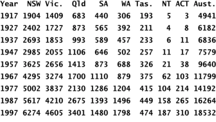
The column names (accessed by names (Cars93.summary)) are Min.passengers (ie the minimum number of ..passengers for cars in this category), Max.passengers, No.cars and county. The return value is the value of the last (and in this case only) expression that appears in the body of the function18.
Plotting
- plot () and allied functions
- Plot methods for other classes of object
- Fine control – Parameter settings
- Multiple plots on the one page
- The shape of the graph sheet
- Adding points, lines and text
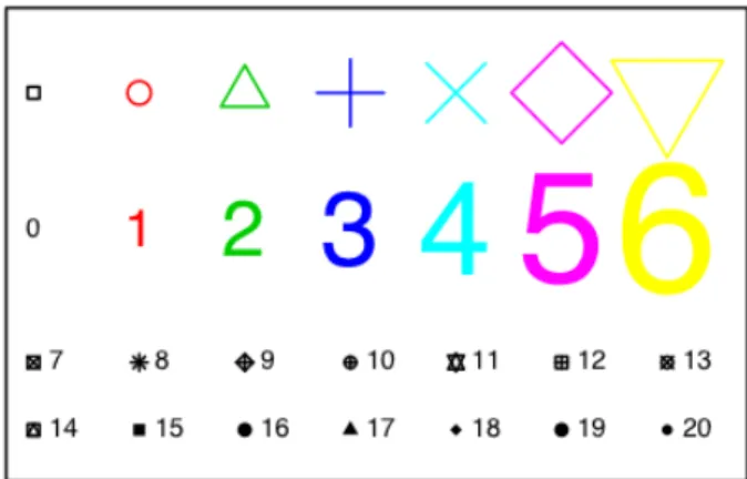
- Size, colour and choice of plotting symbol
- Adding Text in the Margin
- Identification and Location on the Figure Region
- identify()
- locator()
- Plots that show the distribution of data values
- Histograms and density plots
- Boxplots
- Normal probability plots
- Other Useful Plotting Functions
- Scatterplot smoothing
- Adding lines to plots
- Rugplots
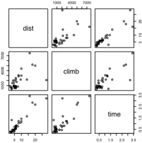
- Scatterplot matrices
- Dotcharts
- Plotting Mathematical Symbols
- Guidelines for Graphs
- Exercises
- References
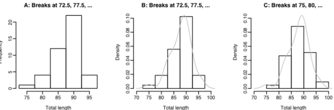
It uses the pos=4 parameter setting to move the labeling to the right of the points. Click to the left or right, and slightly above or below a point, depending on how you want the label positioned. Panel C has a different choice of breakpoints, giving the histogram a rather different impression of the distribution of the data.
In Figure 9B, the y-axis of the histogram is labeled such that the area of a rectangle is the density for that rectangle, i.e. the frequency of the rectangle is divided by the width of the rectangle. The only difference between Figure 9C and Figure 9B is that a different choice of breakpoints is used for the histogram, so the histogram gives a rather different impression of the distribution of the data. By default, carpet(x) adds vertical lines along the x-axis of the current plot that show the distribution of values of x.
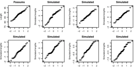
For the first two columns of data frame hills, examine the distribution using: (a) the histogram; (b) density plots; (c) normal probability plots.
Lattice graphics
- Examples that Present Panels of Scatterplots – Using xyplot()
- Some further examples of lattice plots
- Plotting columns in parallel
- Fixed, sliced and free scales
- An incomplete list of lattice Functions
- Exercises
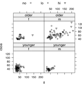
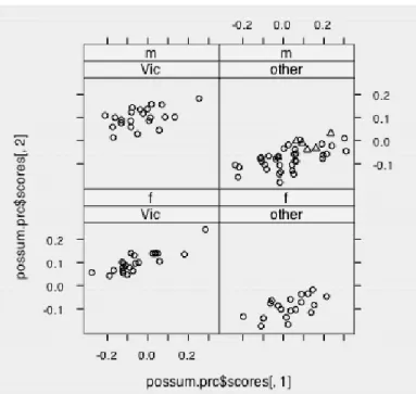
A notable feature is that very high values, both for csoa and for, occur only in older men. The relationship between csoa and it appears very similar for both contrast levels. Finally, we make a drawing (Figure 15) that uses different symbols (black and white) for different levels of coloring.
Use the outer parameter to control whether the columns appear on the same or separate panels. If it is on the same panel, it is desirable to use auto.key to provide a simple key. Use trellis.par.set() to make the changes for the duration of the current device unless reset.
In most cases, a group parameter can be specified, that is, the plot is repeated for the groupings within one panel.
Linear (Multiple Regression) Models and Analysis of Variance
- The Model Formula in Straight Line Regression
- Regression Objects
- Model Formulae, and the X Matrix
- Model Formulae in General
- Multiple Linear Regression Models
- The data frame Rubber
- Weights of Books
- Polynomial and Spline Regression
- Polynomial Terms in Linear Models
- What order of polynomial?
- Pointwise confidence bounds for the fitted curve
- Spline Terms in Linear Models
- Using Factors in R Models
- The Model Matrix
- Multiple Lines – Different Regression Lines for Different Species
- aov models (Analysis of Variance)
- Plant Growth Example
- Exercises
- References
Fit values are given by multiplying each column of the model matrix by its corresponding parameter, i.e. The design of the data set is really important for interpreting coefficients from a regression equation. The increase in the number of degrees of freedom more than compensates for the decrease in the F statistic. gt; # However, we have an independent estimate of the error mean.
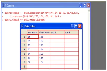
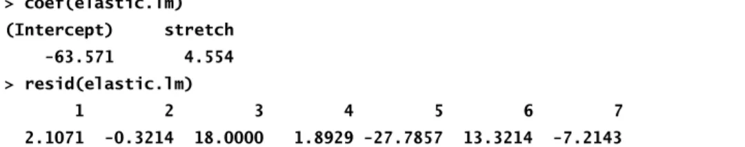
Here we take advantage of this to fit different lines to different subsets of the data. Examination of the plot indicates that cultivars differ greatly in the variation in head weight. For each of the data sets elastic1 and elastic2, determine the regression of elasticity on distance.
Check in section 5.7 the form of the model matrix (i) for the fitting of two parallel lines and (ii) for the fitting of two arbitrary lines when one uses the sum contrasts.
Multivariate and Tree-based Methods
- Multivariate EDA, and Principal Components Analysis
- Cluster Analysis
- Discriminant Analysis
- Decision Tree models (Tree-based models)
- Exercises
- References
- Vectors
- Subsets of Vectors
- Patterned Data
- Missing Values
- Data frames
- Extraction of Component Parts of Data frames
- Data Sets that Accompany R Packages
- Data Entry Issues
- Idiosyncrasies
- Missing values when using read.table()
- Separators when using read.table()
- Factors and Ordered Factors
- Ordered Factors
- Lists
- Arrays
- Conversion of Numeric Data frames into Matrices
- Exercises
Plot a distribution matrix of the first three principal components, using different colors or symbols to identify different schools. The concept of a data frame is essential to using most R modeling and graphics functions. The first column holds the row labels, which in this case are the row numbers that were drawn.
When, as in the above example, one of the columns contains text strings, by default the column is stored as a factor with as many different levels as there are unique text strings35. They provide an economical way to store vectors of character strings where there are many multiple occurrences of the same strings. They are stored as integer vectors, where each of the values is interpreted according to the information in the table of levels38.
Find the average snow cover (a) for the odd years and (b) for the even years.
Functions
Functions for Confidence Intervals and Tests
- The t-test and associated confidence interval
- Chi-Square tests for two-way tables
Matching and Ordering
String Functions
Application of a Function to the Columns of an Array or Data Frame
- apply()
- sapply()
The syntax for tapply() is similar, except that the name of the second argument is INDEX instead of by. If there is no data value for a given combination of factor levels, NA is returned. The Cars93 data frame (MASS package) contains extensive data on 93 cars sold in the United States in 1993.
I've created a data frame Cars93.summary where the row names are the distinct values of Type, while a later column holds two character abbreviations of each of the car types, suitable for use in plotting. This creates a data frame that has the abbreviations in the extra column named "abbrev". If there had been rows with missing values of Type, these would have been omitted from the new data frame.
This can be avoided by ensuring that Type has NA as one of its levels, in both data frames.
Dates
Writing Functions and other Code
- Syntax and Semantics
- A Function that gives Data Frame Details
- Compare Working Directory Data Sets with a Reference Set
- Issues for the Writing and Use of Functions
- Functions as aids to Data Management
- Graphs
- A Simulation Example
- Poisson Random Numbers
In general, the first argument of sapply() can be a list.] To apply faclev() to all mole columns of the data frame, we can specify. Settings that may need to be changed in subsequent use of the function should appear as default settings for the parameters. Often a good strategy is to use default parameters that will serve for a demonstration run of the function.
You can then automatically generate the file names by using paste() to paste the separate parts of the name together. We can simulate the correctness of the student for each question by generating an independent uniform random number. One can think of the Poisson distribution as the distribution of the total for occurrences of rare events.
The total number of accidents during a year may follow a distribution that is close to Poisson.
Exercises
So you can write an R function that simulates a student betting on a True-False test consisting of any number of questions. Write an R function that simulates the number of 500 working bulbs, where each bulb has a 0.99 probability of working. Write a function that performs an arbitrary number n repeated simulations of the number of accidents in a year, and plots the result in a suitable way.
Write a function that simulates the repeated calculation of the coefficient of variation (= the ratio between the mean and the standard deviation), for independent random samples from a normal distribution. Write a function that calculates the median of the absolute values of the deviations from the sample median for each sample. The first element is the number of occurrences of level 1, the second is the number of occurrences of level 2, and so on.
Write a function that calculates the minimum of a quadratic, and the value of the function as the minimum.
A Taxonomy of Extensions to the Linear Model
For example, g(.) can be a function that undoes the logit transformation, as in a logistic regression model. The reason is that g(.) is a specific function such as the inverse of the logit function. Fitting the glue terms (bs() or ns()) in a linear model or a generalized linear model can be a good alternative to using a full generalized additive model.
Logistic Regression
- Anesthetic Depth Example
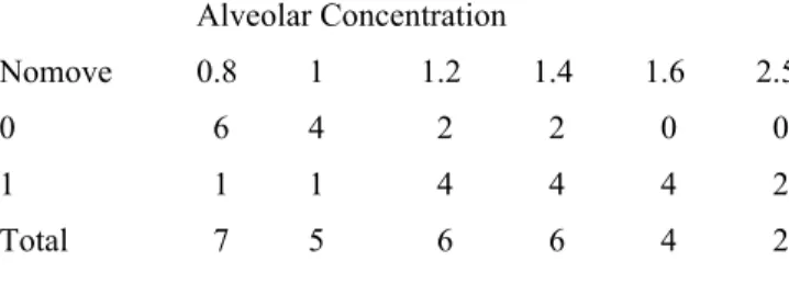
The interest is to assess how the probability of twitching or twisting changes with increasing concentration of the anesthetic agent. We can fit the models either directly to the 0/1 data, or to the proportions in Table 1. 40 I am grateful to John Erickson (Anesthesia and Critical Care, University of Chicago) and Alan Welsh (Center for Mathematics and its Applications , Australian National University) for permission to use this data.
The horizontal line estimates the expected proportion of nominations if concentration had no effect. Null deviation: 41.5 at 29 degrees of freedom Residual deviation: 27.8 at 28 degrees of freedom Number of replicates of Fisher's score: 5. Line is the estimate of the proportion of movements, based on the fitted logit model.
With such a small sample size it is impossible to do much useful to check the suitability of the model.
- Data in the form of counts
- The gaussian family
Models that Include Smooth Spline Terms
- Dewpoint Data
Survival Analysis
Non-linear Models
Model Summaries
Further Elaborations
Exercises
Multi-Level Models, Including Repeated Measures Models
- The Kiwifruit Shading Data, Again
- The Tinting of Car Windows
- The Michelson Speed of Light Data
In section 4.1 we encountered data from an experiment that aimed to model the effects of car window tinting on visual performance42. In this data frame, csoa (critical stimulus onset asynchrony, i.e. the time in milliseconds required to recognize an alphanumeric target), it (inspection time, i.e. the time required for a simple discrimination task) and age are variables, while color (3 levels) and target (2 levels) are ordered factors. Such plots as we examined in section 4.1 make it clear that, to obtain variances that are approximately
This is so that we can do the equivalent of a comparison of variance analysis. Maximum likelihood tests show that at least this complexity of variance and dependence structure is required to accurately represent the data. A model with neither fixed nor random effects of Run appears to be statistically justified.
To test this, one should fit models with and without these effects, setting method=“ML” in each case, and compare the probabilities.
Time Series Models
Exercises
Methods
Extracting Arguments to Functions
Parsing and Evaluation of Expressions
Here is a function that creates a new dataframe from an arbitrary set of columns in an existing dataframe. Once inside the function, we attach the data frame so we can leave out the name of the data frame and just use the column names. The do.call() function allows you to specify the function name and argument list in separate text strings.
When using do.call it is only necessary to use parse() to generate the argument list.
Plotting a mathematical expression
Searching R functions for a specified token
Appendix 1
R Packages for Windows
Contributed Documents and Published Literature
Data Sets Referred to in these Notes
Answers to Selected Exercises