More specifically, stochastic integrals as such result when a stochastic process is integrated with respect to the Wiener process, e.g. Ito integralR. On the one hand, I would like to give a basic and illustrative presentation of the relevant topics without many "difficulties".
Introduction
- Summary
- Finance
- Econometrics
- Mathematics
- Problems and Solutions
The answers to these and similar questions will be found in Chapter 13 on interest rate models. Engle (1982) proposed the so-called ARCH model (see Chapter 6) to capture the bounded effects.
Time Series Modeling
Basic Concepts from Probability Theory
Summary
Random Variables
Example 2.3 (Kurtosis of a continuous uniform distribution) The random variable Xi is assumed to be uniformly distributed over Œ0;bwith density. Example 2.4 (Normal distribution) The density of a random variable X with normal or Gaussian distribution with parameters and > 0 goes back to Gauss5 and is known to be .
Joint and Conditional Distributions
This relationship is similar to (2.2); in fact, both relations are special cases of Jensen's inequality.8 A random variable is called integrable if E.jXj/ <1. This calculation can be performed by applying a rule called the "law of iterated expectations (LIE)" in the literature; it is given in Proposition 2.1.
Stochastic Processes (SP)
SP is called a Markov process if all information from the past about its future behavior is fully concentrated in the present. To capture this concept more precisely, the set of information about the history of a process available up to a time is denoted by It.
Problems and Solutions
In particular, it can be observed that the expression is always positive except for the case Y DZ. For the third equality, the order of integration is reversed; this is because of Fubini's statement.
ARMA)
Summary
Moving Average Processes
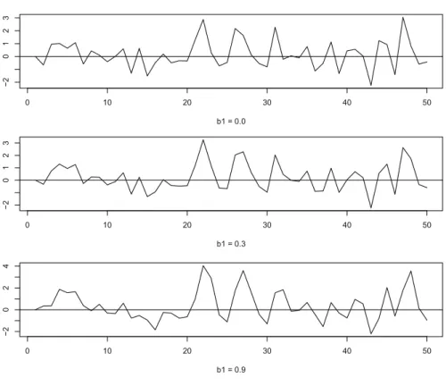
46 3 Autoregressive Moving Average Processes (ARMA) Since the innovations are WN.0; 2/, the moments are independent of time: First, it applies that E.xt/DD0. Proposition 3.2 (infinite MA) Assume an MA(1) process, xt DC. a) The process is stationary with expected value and for the autocovariances it holds.
Lag Polynomials and Invertibility
By expressing the filters using the shift operator, they can be manipulated just like ordinary (complex-valued) polynomials. To do this, we define the so-called z-transform of the lag polynomial, where zbe is an element of the complex numbers (z2C):A1.z/D1 az. This invertibility condition for A1.L/ from (3.8) can easily be transferred to the polynomial P.L/ of order p.
Autoregressive and Mixed Processes
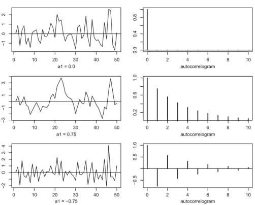
Therefore, the zero line is crossed more often than in the first case of no serial correlation. For max.p;qC1/ the autocorrelations satisfy the same difference equation as in the pure AR(p) case. Before turning to the ARMA(1,1) case, we note that an analogous result to Theorem 3.5(a) is available for an AR(1) representation according to Theorem 3.3: The ARMA process has an absolutely addable AR(1) representation (see Example 3.3) if and only if . B.z/D0 ) jzj> 1 : In this case the ARMA process is called invertible.
Problems and Solutions
As stated, the solution of the difference equation thus obtained (˛j D a˛j 1) is clearly ˛jDaj. By (3.16) there is an even number of positive and negative roots, so that the requested claim also follows from (3.15). 2) Odd degree: because an oddpone also obtains the requested result by distinguishing between the two cases for the sign ofap. AsxtC can be expressed as a function of xtC tCsalone, the further past of the process does not matter for the conditional distribution of xtCs.
Spectra of Stationary Processes
Summary
Definition and Interpretation
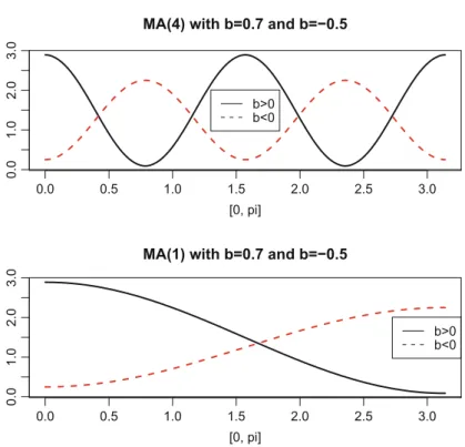
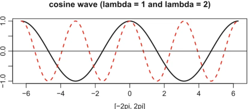
This equation means: the spectrum at0 measures how strongly the cycle with frequency0 and therefore the period P0 D 2=0 adds to the variance of the process. In Figure 4.2, we find two characteristic forms of the spectrum of the MA seasonal process for 5 S D 4 (quarterly data) with b D 0:7 and b D 0:5. And vice versa, for b < 0 it is true that these very cycles add little to the variance of the process.
Filtered Processes
If F.L/ is a finite filter (i.e. with finitep), then the sums of TF./ are truncated accordingly, see (4.8) in the next section. We now return more systematically to the issue of persistence that we touched on in the previous chapter in the example of the AR(1) process. In the previous chapter we mentioned that it has been proposed to measure persistence through the cumulative impulse responses CIR defined in (3.3).
Examples of ARMA Spectra
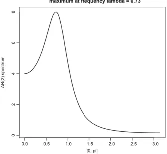
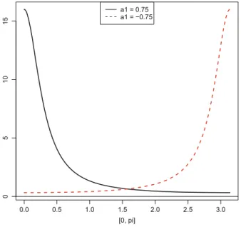
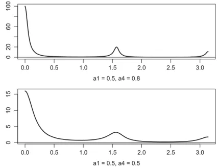
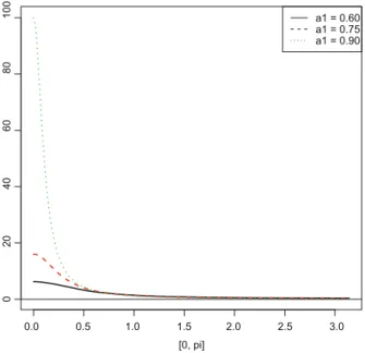
In problem 4.4, we will show that there are extrema at D0 and D where the slope of the spectrum is zero. In fig. 4.6, spectra for four parameter constellations are depicted; these are exactly the four cases for which autocorrelograms are given in Fig.3.4. The spectrum in the lower left is even more extreme: apart from a rather small area around D 2 , it is zero almost everywhere, so there is no trend component.
Problems and Solutions
Discuss its behavior especially for the MA(1) model (compared to the AR(1) case given in (4.7)). For b > 0, the sequence of extrema starts with a maximum at zero; forb < 0, we get a minimum, vice versa. Therefore, the MA(1) invertible process with jb1j < 1 can capture only very moderate persistence compared to the AR(1) case where VR grows with a1 beyond any limit.
Long Memory and Fractional Integration
Summary
Persistence and Long Memory
Unlike the exponential case typical of ARMA processes, hyperbolic decay is so slow for positive d > 0, that the impulse responses are not addable. For a process to be stationary, we require the impulse-response sequence to be quadratic addable, see Theorem 3.2. 108 5 Long Memory and Fractional Integration Fractional integration thus imposes the hyperbolic decay rate discussed above, where the rate of convergence varies with .
Fractionally Integrated Noise
110 5 Long Memory and Fractional Integration from the hyperbolic decomposition of the autocovariance sequence we note that.h/. More precisely, Proposition 5.1(c) says for any finite that the autocorrelation increases with d(ford > 0), which reinforces the interpretation of the measure of persistence or long memory.4. It is clear from the definition of the spectrum in (4.3) that it does not exist at the origin under long memory (d > 0), because the autocovariances are not summed.
Generalizations
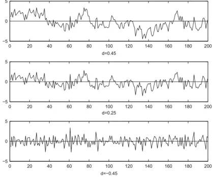
The absolute summability offbkgrules out long memory (word> 0) by the fact that the autocovariances offtegare are absolutely summable, see Proposition 3.2; the second condition that the sequence fbkg does not sum up to zero rules out that fetgis integrated by orderedwithd< 0, see (5.7). Since fytgis is given by integration over anI.ı/process, we say that fytgis is integrated by orderd,yt I.d/, withd D ıC1. Example 5.2 (Non-stationary fractional noise) The middle graph in fig. 5.6 shows a realization of a random walk (dD1).
Problems and Solutions
120 5 Long memory and fractional integration First we discuss the case that separates the convergence region from the divergent one .pD1/. 124 5 Long memory and fractional integration where the so-called psi function is defined as logarithmic derivative of the Gamma function,. An introduction to long-memory time series models and fractional difference.Journal of Time Series Analysis, 1, 15–29.
Heteroskedasticity (ARCH)
Summary
Time-Dependent Heteroskedasticity
Recall the definition of the information set It 1 generated by the past of xt op toxt 1. The variance of the martingale difference is determined as follows (asxtis zero in average,. For each point in time tone average over the previous previous B values in order for to determine the variance int.
ARCH Models
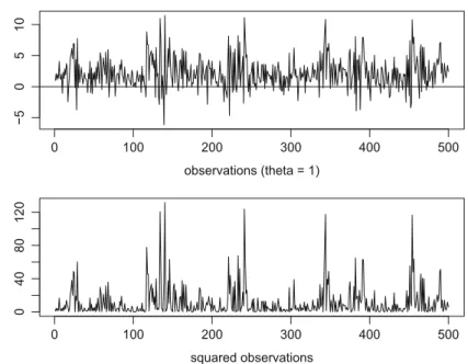
These volatility clusters become even more apparent in the respective lower panels of the figures, in which the squared observations fx2tg are depicted. In the first section of the chapter on basic concepts from probability theory, we defined the kurtosis by means of the fourth moment of a random variable and we denoted the corresponding coefficient by2. For2 > 3 the density function is more "peaked" than the one from the normal distribution: On the one hand the.
Generalizations
We speak of "GARCH in the mean"3(GARCH-M) if the volatility term affects the (mean) level of the process. We speak of exponential GARCH when volatility is modeled as an exponential function of the squares of the pastx2t i. When comparing the graphs of the squared observations and the original ones, it can be found that they are more extreme amplitudes.
Problems and Solutions
144 6 Processes with autoregressive conditional heteroskedasticity (ARCH) where the assumption for the last inequality was used. Therefore, we have shown for a rootzof˛.z/ that it holds that maxjjzjj> 1and thusjzj> 1. To determine the kurtosis, we first observe that the fourth moment is constant under the condition 3˛12 < 1.
Stochastic Integrals
Wiener Processes (WP)
Summary
From Random Walk to Wiener Process
Since it depends on the choice of n (i.e. the fineness of the partition), the process Xn.t/ is indexed accordingly. At the same time, the step height of the steps becomes flatter by n 0:5 the finer it is distributed. More precisely, the WP is even a Gaussian process in the sense of the definition in Chapter 2.
Properties
To show this, we use the fact that the increment W.tCs/ W.t/fors> 0 is independent of the information set It due to (W2). The trend behavior of the non-stationary Wiener process will now be clarified by two theorems. This proves statement (a) from the following statement; statement (b) is obtained by means of the corresponding density function (see Problem 7.5).
![Fig. 7.2 Simulated paths of the WP on the interval [0,1]](https://thumb-ap.123doks.com/thumbv2/123dok/9205883.0/172.659.119.544.93.463/fig-simulated-paths-wp-interval.webp)
Functions of Wiener Processes
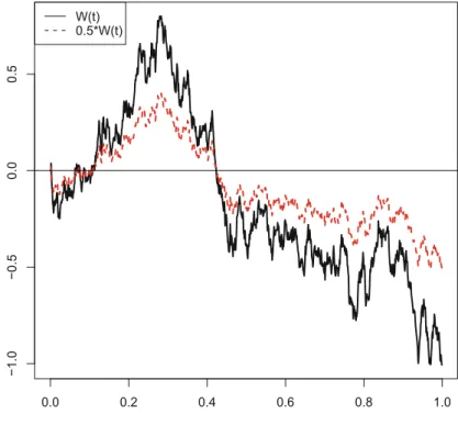
In Fig.7.3 a path of a WP and a Brownian motion based on it with only half the standard deviation. By definition, in this case the logarithm8 of the process is a Brownian motion with drift, and therefore Gaussian. In Fig.7.8 we find graphs of the WP and a geometric Brownian motion with expectation one, namely with D 0:5 and D 1.
Problems and Solutions
By substitution, these moments can be reduced to the Gamma function, which was introduced in Problem 5.3, see also below Eq. Recall the random variable Tbfrom Proposition7.1 specifying the point in time at which W.t/hits the value b for the first time. The event max0stW.s/ < bis equivalent to the fact that the hit time is greater than.
Summary
Definition and Fubini’s Theorem
Further elaborations of mean square convergence can be found at the end of the chapter. A sufficient condition for the existence of the Riemann integral is that the function f is continuous and that in addition E.X.s/X.r// is continuous in both arguments. Adapted to our problem of the expected value of a Riemann integral, the corresponding conditions are given in the following theorem, also Eq.
Riemann Integration of Wiener Processes
Note that the finiteness of the variance expression from Proposition8.3 is precisely sufficient and necessary for the existence of the Riemann integral (Proposition8.1). Therefore, it suggests itself not only to determine the variance as in Proposition 8.3, but also the covariance function. The proof of (c) forc D 0 is given in problem 8.5; for an arbitrary one, the proof is basically the same, but it becomes computationally more involved.
Convergence in Mean Square
Thus, the normality of (b) can be proved only in connection with Stieltjes integrals (see problem 9.2).