13
VALUING COMPANIES
Introduction The two skills Valuation using net asset value Income flow is the key Dividend valuation methods How do you estimate future growth?
Price–earnings ratio model
Valuation using cash flow
Valuing unquoted shares
Unusual companies
Managerial control changes the valuation
Conclusion
Introduction
Managers must become acquainted with the main influences on the valuation of entire companies and how to value individual shares in companies. If they are to be given the responsibility of maximizing the wealth of shareholders managers need knowledge of the factors influencing that wealth, as reflected in the share price of their own company. Without this understanding they will be unable to determine the most important consequence of their actions – the impact on share value. Managers need to appreciate share price derivation because the change in their company’s share value is one of the key factors by which they are judged. It is also useful for them to know how share prices are set if the firm plans to gain a flotation on a stock exchange, or when it is selling a division to another firm. In mergers an acquirer needs good valuation skills so as not to pay more than necessary, and a seller needs to ensure that the price is fair.
This chapter describes the main methods of valuing shares: net asset value, dividend valuation models, price earnings ratio models and cash flow models.
There is an important subsection in the chapter that shows how the valuation of shares differs if the purchase would give managerial control from the valuation of shares which provide only a small minority stake.
The two skills
Two skills are needed to be able to value shares. The first is analytical ability, to be able to understand and use mathematical valuation models. Second, and most importantly, good judgment is needed, because the majority of the inputs to the mathematical calculations are factors, the precise nature of which cannot be defined with absolute certainty, so great skill is required to produce reason- ably accurate results. The main problem is that the determinants of value occur in the future, for example future cash flows, dividends or earnings.
The monetary value of an asset is what someone is prepared to pay for it.
Assets such as cars and houses are difficult enough to value with any degree of accuracy. At least corporate bonds generally have a regular cash flow (coupon) and an anticipated capital repayment. This contrasts with the uncertainties associated with shares, for which there is no guaranteed annual payment and no promise of capital repayment. The difficulties of share valuation are amply represented by the case of Amazon.com in case study 13.1.
Managers need to appreciate share price derivation because the change in their company‘s share value is one of the key factors by which they are judged.
The monetary value of an asset is what someone is prepared to pay for it.
Valuation using net asset value (NAV)
The balance sheet seems an obvious place to start when faced with the task of valuation. In this method the company is viewed as being worth the sum of the value of its net assets. The balance sheet is regarded as providing objective facts concerning the company’s ownership of assets and obligations to creditors. Here fixed assets are recorded along with stocks, debtors, cash and other liquid assets. With the deduction of long-term and short-term creditors from the total asset figure we arrive at the net asset value (NAV).
An example of this type of calculation is shown in Table 13.1 for Cadbury Schweppes.
The NAV of over £3bn of Cadbury Schweppes compares with a market value placed on all the shares when totaled of £8.5bn (market capitalization figures are available in Monday editions of the Financial Times). This great difference makes it clear that the shareholders of Cadbury Schweppes are not rating the firm on the basis of balance sheet net asset figures. This point is emphasized by an examination of Table 13.2.
Three of the four firms listed in Table 13.2 have very small balance sheet values in comparison with their total market capitalization. The exception is Vodafone which boosted its balance sheet by buying many other companies pro- ducing over £90bn intangible assets in the form of goodwill (amount paid for target above the fair value of the assets acquired).
For most companies, investors look to the income flow to be derived from a holding. This flow is generated when the balance sheet assets are combined with assets impossible to quantify: these include the unique skills of the work-
Amazon.com
Amazon, the internet retailer, has never made a profit. In fact it lost over $700m in 1999 and offered little prospect of profits in the near term. So, if you were an investor in early 2000 what value would you give to a company of this caliber? Anything at all? Amazingly, investors valued Amazon at over $30bn in early 2000 (more than all the traditional book retailers put together).
The brand was well established and the numbers joining the online community rose by thou- sands every day. Investors were confident that Amazon would continue to attract customers and produce a rapid rate of growth in revenue. Eventually, it was thought, this revenue growth would translate into profits and high dividends. When investors had calmed down after taking account of the potential for competition and the fact that by 2001 Amazon was still not produc- ing profits, they reassessed the value of Amazon’s likely future dividends. In mid-2001, they judged the company to be worth only $4bn – it had run up losses of $1.4bn in 2000, indicating that profits and dividends were still a long way off. However by 2004 the company, despite reporting yet another loss in 2003, was thought to be close to being able to turn its brand into profits for shareholders, so it was valued at over $20bn. Maybe it will.
Case study 13.1
force, the relationships with customers and suppliers, the value of brands, the reservoir of experience within the management team, and the competitive posi- tioning of the firms’ products. Assets, in the crude sense of balance sheet values, are only one dimension of overall value. Investors in the market generally value intangible, unmeasurable assets more highly than those that can be identified and recorded by accountants.
Criticizing accountants for not producing balance sheets which reflect the true value of a business is unfair. Accounts are not usually designed to record up-to-date market values.
Land and buildings are frequently shown at cost rather than market value; thus TABLE 13.1
Cadbury Schweppes Abridged Balance Sheet 29 December 2002
£m
Fixed assets 5,815
Current assets
Stocks 528
Debtors falling due within one year 970 Debtors falling due after more than one year 82
Investments 297
Cash at bank and in hand 175
––––
2,052 Creditors: Amounts falling due within one year (2,585) Creditors: Amounts falling due after more than one year (1,577)
Provisions for liabilities and charges (419)
–––––––
Net assets 3,286
–––––––
Shareholders’ funds 3,020
Source: Cadbury Schweppes plc Report & Accounts 2002
TABLE 13.2
Net asset values and total capitalization of some firms
Company (Accounts year) NAV £m Total capitalization (market value of company’s shares) £m
GlaxoSmithKline (2002) 7,388 77,306
Unilever (2002) 3,816 29,764
EMI (2002) Negative 889 1,305
Vodafone (2002) 133,428 95,109
Source: Annual reports and accounts;Financial Times, 5 January 2004
Investors in the market generally value intangible, unmeasurable assets more highly than those that can be identified and recorded by accountants.
the balance sheet can provide a significant over- or under-valuation of these assets’ current value. Plant and machinery is shown at the purchase price less a depreciation amount. Stock is valued at the lower of cost or net realizable value – this can lead to a significant under-estimate, as the market value can appreci- ate to a figure far higher than either of these. The list of balance sheet entries vulnerable to subjective estimation, arbitrary method and even cynical manipu- lation is a long one: goodwill, provisions, merger accounting, debtors, intangible brand values and so on.
The slippery concept of balance sheet value is demonstrated in the article about Hanson reproduced in Exhibit 13.1.
When asset values are par ticularly useful
The accounts-based approach to share value is fraught with problems but there are circumstances in which asset backing is correctly given more attention.
Firms in financial difficulty
The shareholders of a firm in financial difficulty may pay a great deal of attention to the asset backing of the firm. They may weigh up the potential for asset sales or asset-backed borrowing. In extreme circumstances they may try to assess the break-up value.
Takeover bids
In a takeover bid shareholders will be reluctant to sell at less than NAV even if the prospect for income growth is poor. A standard defensive tactic in a takeover battle is to revalue balance sheet assets to encourage a higher price.
Income flow Focus of investor’s
attention
Combined with Assets in
balance sheet
Assets which cannot be objectively measured, e.g.
• the reservoir of experience within the management team
• the unique skills of the workforce
• relationships with suppliers
FIGURE 13.1
What creates value for shareholders?
When discounted income flow techniques are difficult to apply
For some types of company there is no straightforward way of employing income-flow based methods:
Property investment companies
These are primarily valued on the basis of their assets. It is generally possible to put a fairly realistic up-to-date price on the buildings owned by such a company.
These market values have a close link to future cash flows. That is, the future rents payable by tenants, when discounted, determine the value of property assets and thus the company. If higher rent levels are expected than were previ- ously anticipated, chartered surveyors will place a higher value on the asset, and the NAV in the balance sheet will rise, forcing up the share price. For such com- panies, future income, asset values and share values are all fairly closely linked.
However, as Exhibit 13.2 makes clear, while share price and NAV generally go up and down together, there are good reasons for property investment company shares to trade at less than NAV.
EXHIBIT 13.1 Hanson cuts asset value
Source: Financial Times9 July 1996
Hanson cuts asset value by £3.2bn
Tim Burt
Hanson, the industrial conglomerate, yesterday marked the latest stage of its four-way demerger by announcing a
£3.2bn reduction in assets following accounting changes and write-downs in the value of its US mineral reserves.
The write-downs at Peabody, the largest coal producer in the US, and Hanson’s Cornerstone aggregates sub- sidiary will bring the company into line with US accounting standards on the treatment of ‘long lived assets’.
Mr Derek Bonham, chief executive, said the move would have no impact on operational cash flow and added: ‘It in no way reflects on the accuracy of pre- vious accounts.’
Some industry analysts, however, suggested Hanson might have overval-
ued the assets of both Peabody and Cornerstone in the past – a charge rejected by the company.
In total, the book value of mineral reserves at Cornerstone have been reduced by £2.3bn to £1.3bn and by
£600m at Peabody to £1.5bn. A further
£300m charge is being made against Peabody’s reserves to cover accounting changes over industry liabilities.
As part of the accounting changes, Hanson has removed £1.2bn of its
£1.5bn provisions from Peabody’s bal- ance sheet and plans to charge £300m of previous payments to profit and loss reserves. Mr Bonham said this move would cut the carrying value of Peabody’s coal reserves by £1.5bn.
Investment trusts
The future income of investment trusts comes from the individual sharehold- ings. The shareholder in a trust would find it extremely difficult to calculate the future income to be received from each of the dozens or hundreds of shares held. An easier approach is simply to take the current share price of each hold- ing as representing the future discounted income. The share values are aggregated to derive the trust’s NAV and this has a strong bearing on the price at which the trust shares are traded.
EXHIBIT 13.2 When net asset value is no guide
Source:Financial Times17 August 2001
When net asset value is no guide
Norma Cohen
The directors of Asda Property face a dilemma – do they recommend sharehold- ers to accept a bid that is significantly below the company’s ‘value’ or do they urge them to accept it on the grounds that it is the best offer they are likely to get?
If the offer is accepted, what does the concept of net asset value really mean?
If the offer is rejected, does that mean NAV is a concept that has no rele- vance to share price?
Last week, the directors – not includ- ing the executive chairman and founder, Manny Davidson – initiated a ‘first’ for the quoted property sector, seeing off a bid approach of 280p that was deemed too low. Similar bids for other property companies have been accepted almost without question.
But yesterday’s renewed offer of 298.6p, along with the latest 1.4p interim dividend, now requires pause for thought. Asda’s current situation is awkward. …
… In rejecting the initial offer, Asda’s directors point to the latest interim val- uation of 383p, including 6p on the development portfolio.
In justifying its offer, BL Davidson, the joint venture, points to the 60p per share capital gains tax the company would incur on the sale of its assets,
along with further deductions for paying off high interest rate debt. After these deductions, NAV falls to 308p, not far off its offer price. …
… But if a company is not to be valued at its break-up value, what sort of price should you put on it?
NAV is an interesting number because, in its pure form, it takes no account of the break-up costs. But equally, it takes no account of the cost of remaining a going concern.
Indeed, NAV is a number that pre- tends there is no cost associated with corporate ownership and management of real estate – a patent nonsense.
For one thing, there are general overhead and administrative costs; for another, there is depreciation expense.
Although the latter never appears in corporate profit and loss accounts, there is ample evidence it exists.
Unrecoverable property management and refurbishment costs are, in effect, disguised forms of depreciation expense.
A more ‘true’ picture would emerge if analysts could count the net present value of those costs and deduct them from the NAV.
Arguably, this is what the market does already. Indeed, it may explain the staggering range of discounts to NAV at which property company shares trade.
Resource-based companies
For oil companies, mineral extractors, mining houses and so on, the proven or prob- able reserves have a significant influence on the share price (seeExhibit 13.3).
Income flow is the key
The value of a share is usually determined by the income flows that investors expect to receive in the future from its ownership. Information about the past is only of relevance to the extent that it contributes to an understanding of expected future performance. Income flows will occur at different points in the future and so they have to be discounted. There are three classes of income val- uation models:
■ dividend-based models
■ earnings-based models
■ cash flow-based models.
Dividend valuation methods
The dividend valuation models (DVMs) are based on the premise that the market value of ordinary shares represents the sum of the expected future dividend flows, to infinity, discounted to present value.
The only cash flows that investors ever receive from a company are dividends.
This holds true if we include a ‘liquidation dividend’ upon the sale of the firm or on formal liquidation, and any share repurchases can be treated as dividends. Of
EXHIBIT 13.3 NAV valuation sparks dispute
Source: Investors Chronicle, 11 June 1999
NAV valuation sparks dispute
Timon Day
A row had broken out between oil com- pany LASMO and HSBC Securities over the broker’s sharp cut in its estimation of LASMO’s net asset value from 132p to 98p a share. It knocked £48m off LASMOs stock market value driving its shares down 5p to 123p. This is a par- ticularly sensitive time because LASMO is in the middle of an all-share offer for Monument Oil & Gas – whose former broker is HSBC …
Most of the dispute over the valua- tion centres on Algeria where LASMO has a 12 per cent stake in 14 oil fields operated by US group Anadarko. Mr Perry does not accept LASMO’s valua- tion of between £300m and £500m for its Algerian interests, putting a price of just £210m on them.
course, an individual shareholder is not planning to hold a share forever to gain the dividend returns to an infinite horizon. An individual holder of shares will expect two types of return:
■ income from dividends and
■ a capital gain resulting from the appreciation of the share and its sale to another investor.
The fact that the individual investor is looking for capital gains as well as divi- dends to give a return does not invalidate the models’ focus on all dividends to an infinite horizon. The reason for this is that when a share is sold by that investor, the purchaser is buying a future stream of dividends, so the price paid is determined by future dividend expectations.
To illustrate this, consider the following: A shareholder intends to hold a share for one year. A single dividend will be paid at the end of the holding period, d1and the share will be sold at a price P1in one year.
To derive the value of a share at time 0 to this investor (P0), the future cash flows, d1and P1, have to be discounted at a rate which includes an allowance for the risk class of the share, kE.
d1 P1 P0= –––––– + –––––––
1 + kE 1 + kE
The dividend valuation model to infinity
The relevant question to ask to understand DVMs is: Where does P1come from?
The buyer at time 1 estimates the value of the share based on the present value of future income given the required rate of return for the risk class. So if the second investor expects to hold the share for a further year and sell at time 2 for P2, the price P1will be:
d2 P2 P1= –––––– + ––––––
1 +kE 1 + kE Example
An investor is considering the purchase of some shares in Willow plc. At the end of one year a dividend of 22p will be paid and the shares are expected to be sold for
£2.43. How much should be paid if the investor judges that the rate of return required on a financial security of this risk class is 20 percent?
Answer
d1 P1 P0= –––––– + –––––
1 + kE 1 + kE
22 243
P0= ––––––– + ––––––– = 221p 1 + 0.2 1 + 0.2
Returning to the P0equation we are able to substitute discounted d2and P2 for P1. Thus:
d1 P1 P0= –––––– + ––––––
1 + kE 1 +kE
d1 d2 P2
P0= –––––– + –––––––– + ––––––––
1 +kE (1 +kE)2 (1 +kE)2
If a series of one-year investors bought this share, and we in turn solved for P2, P3, P4, etc., we would find:
d1 d2 d3 dn
P0= –––––– + –––––––– + ––––––––– + … + ––––––––
1 +kE (1 +kE)2 (1 +kE)3 (1 +kE)n
Even a short-term investor has to consider events beyond his or her time hori- zon because the selling price is determined by the willingness of a buyer to purchase a future dividend stream. If this year’s dividends are boosted by short- termist policies such as cutting out R&D and brand-support marketing the investor may well lose significantly because other investors push down the share price as their forecasts for future dividends are lowered.
The dividend growth model
In contrast to the situation in the above example, for most companies dividends are expected to grow from one year to the next.1To make DVM analysis manage- able simplifying assumptions are usually made about the patterns of growth in dividends. Most managers attempt to make dividends grow more or less in line with the firm’s long-term earnings growth rate. They often bend over backwards
Example
If a firm is expected to pay dividends of 20p per year to infinity and the rate of return required on a share of this risk class is 12% then:
20 20 20 20
P0= –––––––– + –––––––––– + –––––––––– + … + ––––––––––
1 + 0.12 (1 + 0.12)2 (1 + 0.12)3 (1 + 0.12)n P0= 17.86 + 15.94 + 14.24 + … + … +
Given this is a perpetuity there is a simpler approach:
d1 20
P0= ––– = –––– = 166.67p kE 0.12
to smooth out fluctuations, maintaining a high dividend even in years of poor profits or losses. In years of very high profits they are often reluctant to increase the dividend by a large percentage for fear that it
might have to be cut back in a downturn. So, given management propensity to make dividend payments grow in an incremental or stepped fashion it seems that a reasonable model could be based on the assumption of a constant growth rate. (Year to year deviations around this expected growth path will not materially alter the analysis.)
Given management propensity to make dividend payments grow in an incremental or stepped fashion it seems that a reasonable model could be based on the assumption of a constant growth rate.
Worked example 13.1
A CONSTANT DIVIDEND GROWTH VALUATION: SHHH PLC If the last dividend paid was d0and the next is due in one year, d1, then this will amount to d0(1 + g) where gis the growth rate of dividends.
For example, if Shhh plc has just paid a dividend of 10p and the growth rate is 7% then:
d1will equal d0(1 + g) = 10 (1 + 0.07) = 10.7p and
d2will be d0(1 + g)2= 10 (1 + 0.07)2= 11.45p
The value of a share in Shhh will be all the future dividends discounted at the risk-adjusted discount rate of 11%:
d0(1 + g) d0(1 + g)2 d0(1 + g)3 d0(1 + g)n P0= ––––––––– + –––––––––– + –––––––––– + … + –––––––––
1 + kE (1 + kE)2 (1 + kE)3 (1 + kE)n
10(1 + 0.07) 10(1 + 0.07)2 10(1 + 0.07)3 d0(1 + g)n P0= –––––––––––– + ––––––––––––– + –––––––––––– + … + ––––––––––
1 + 0.11 (1 + 0.11)2 (1 + 0.11)3 (1 + kE)n Using the above formula could require a lot of time. Fortunately it is mathematically equivalent to the following formula,2 which is much easier to employ.
d1 d0(1 + g) 10.7
P0= –––––– = ––––––––– = –––––––––– = 267.50p kE– g kE– g 0.11 – 0.07
Note that, even though the shortened formula only includes next year’s dividend all the future dividends are represented.
A further illustration is provided by the example of Pearson plc.
Non-constant growth
Firms tend to go through different phases of growth. If they have a strong com- petitive advantage in an attractive market they might enjoy super-normal growth. Eventually, however, most firms come under competitive pressure and growth becomes normal. Ultimately, many firms fail to keep pace with the market environmental change in which they operate and growth falls to below that for the average company.
To analyze companies that go through different phases of growth a two-, three- or four-stage model may be used. In the simplest case of two-stage growth the share price calculation requires the adding together of the results of the following:
Worked example 13.2 PEARSON PLC
Pearson plc, the publishing, media and education group, has the following dividend history:
The average annual growth rate, g, over this period has been:
g= 6 –––– – 1 = 0.064 or23.4 6.4%
16.1
If it is assumed that this historic growth rate will continue into the future and 10% is taken as the required rate of return, the value of a share can be calculated.
d1 23.4(1 + 0.064)
P0= –––––– = ––––––––––––––– = 692p kE– g 0.10 – 0.064
In fact, in early 2004 Pearson’s shares stood at 620p. Perhaps analysts were anticipating a slower rate of growth in future than in the past.
Perhaps we employed an unreasonably low discount rate given the risks facing the company. Or perhaps the market consensus view of Pearson’s growth prospects was over-pessimistic.
Year Net dividend per share (p)
1996 16.1
1997 17.4
1998 18.8
1999 20.1
2000 21.4
2001 22.3
2002 23.4
■ Discount each of the forecast annual dividends in the first period to time 0.
■ Estimate the share price at the point at which the dividend growth shifts to the new permanent rate. Discount this share price to time 0.
Worked example 13.3 NORUCE PLC
You are given the following information about Noruce plc.
The company has just paid an annual dividend of 15p per share and the next is due in one year. For the next three years dividends are expected to grow at 12% per year. This rapid rate is caused by a number of favorable fac- tors: an economic upturn, the fast acceleration stage of newly developed products and a large contract with a government department.
After the third year the dividends will grow at only 7% per annum, because the main boosts to growth will, by then, be absent.
Shares in other companies with a similar level of systematic risk to Noruce produce an expected return of 16% per annum.
What is the value of one share in Noruce plc?
Answer
Stage 1 Calculate dividends for the super-normal growth phase.
d1= 15(1 + 0.12) = 16.8 d2= 15(1 + 0.12)2 = 18.8 d3= 15(1 + 0.12)3 = 21.1
Stage 2 Calculate share price at time 3 when the dividend growth rate shifts to the new permanent rate.
d3(1 + g) 21.1(1 + 0.07)
P3= ––––––––– = –––––––––––––– = 250.9 kE– g 0.16 – 0.07
Stage 3 Discount and sum the amounts calculated in Stages 1 and 2.
d1 16.8
–––––– = –––––––– = 14.5 1 + kE 1 + 0.16
d2 18.8
+ ––––––––– = –––––––––– = 14.0 (1 + kE)2 (1 + 0.16)2
d3 21.1
+ ––––––––– = ––––––––––– = 13.5 (1 + kE)3 (1 + 0.16)3
P3 250.9
+ ––––––––– = –––––––––– = 160.7 (1 + kE)3 (1 + 0.16)3 –––––––
202.7p
What is a normal growth rate?
Growth rates will be different for each company but for corporations taken as a whole dividend growth will not be significantly different from the growth in nom- inal gross national product (real GNP plus inflation) over the long term. If dividends did grow in a long-term trend above this rate then they would take an increasing proportion of national income – ultimately squeezing out the con- sumption and government sectors. This is, of course, ridiculous. Thus, in an economy with expected long-term inflation of 3 percent per annum and growth of 2.5 percent, we might expect the long-term growth in dividends to be about 5.5 percent. Also, it is unreasonable to suppose that a firm can grow its earnings and dividends forever at a rate significantly greater than that for the economy as a whole. To do so is to assume that the firm eventually becomes larger than the economy. There will be years, even decades, when average corporate dividends do grow faster than the economy as a whole and there will always be companies with much higher projected growth rates than the average for periods of time.
Nevertheless the real GNP + inflation growth relation- ship provides a useful benchmark.
Companies that do not pay dividends
Some companies, for example Warren Buffett’s Berkshire Hathaway, do not pay dividends. This is a deliberate policy as there is often a well-founded belief that the funds are better used within the firms than they would be if the money is given to shareholders. This presents an apparent problem for the DVM but the measure can still be applied because it is reasonable to suppose that one day these companies will start to pay dividends. Perhaps this will take the form of a final break-up payment, or perhaps when the founder is approaching retirement he/she will start to distribute the accumulated resources. At some point divi- dends must be paid, otherwise there would be no attraction in holding the shares. Microsoft is an example of a company that did not pay a dividend for 28 years. However, in 2003 it decided that it would start a process of payout of some of its enormous pile of cash – seeExhibit 13.4.
Some companies do not pay dividends for many years due to regular losses.
Often what gives value to this type of share is the optimism that the company will recover and that dividends will be paid in the distant future.
Problems with the dividend growth valuation model Dividend valuation models present the following problems.
1 They are highly sensitive to assumptions. Take the case of Pearson above. If we change the growth assumption to 7 percent and reduce the required rate of return to 9.5 percent, the value of the share leaps to over £10.
d1 23.4(1 + 0.07)
P0= –––––– = –––––––––––––– = 1002p KE– g 0.095 – 0.07
There will be years, even
decades, when average corporate dividends do grow faster than the economy as a whole.
2 The quality of input data is often poor. The problems of calculating an appropriate required rate of return on equity are discussed in Chapter 10.
Added to this is great uncertainty about the future growth rate.
3 If g exceeds kEa nonsensical result occurs. This problem is dealt with if an assumption of a short-term super-normal growth rate followed by a lower rate after the super-normal period is replaced with a g which is some weighted average growth rate reflecting the return expected over the long run. Alternatively, for those periods when gis greater than k, one may calcu- late the specific dividend amounts and discount them as in the non-constant growth model. For the years after the super-normal growth occurs, the usual growth formula may be used.
The difficulties of using the DVMs are real and yet the methods are to be favored, less for the derivation of a single number than for the understanding of the principles behind the value of financial assets that
the exercise provides. They demand a disciplined thought process that makes the analyst’s assumptions about key variables explicit.
How do you estimate future growth?
The most influential variable, and the one subject to most uncertainty, on the value of shares is the growth rate expected in dividends. Accuracy here is a much sought-after virtue. While this book cannot provide readers with a perfect crystal ball for seeing future dividend growth rates, it can provide a few pointers.
Exhibit 13.4Microsoft considers dividend
Source: Financial Times4 July 2003
Microsoft considers dividend of $10bn-plus
By Emmanuel Paquettein Paris and Richard Watersin San Francisco
Microsoft is considering paying its shareholders a special dividend of ‘sig- nificantly’ more than $10bn (£6bn), according to a person close to the dis- cussions. This would be the largest corporate pay-out ever, and help reduce its $46bn cash pile. …
The software giant has come under increasing pressure from shareholders to release some of its cash pile which has grown as its shares have lagged. A deci- son made to begin paying a dividend,
which will amount to nearly $900m this year, will make little impact as it contin- ues to generate $3bn of cash each quarter. …
The company said when it originally announced its 8 cents per share divi- dend – the first paid in its 28-year history – that it would consider raising the pay-out. One option would involve distributing more than $1 per share at a cost of more than $10bn.
DVMs demand a disciplined thought process that makes the analyst’s assumptions about key variables explicit.
Determinants of growth
Three factors influence the rate of dividend growth.
■ The quantity of resources retained and reinvested within the business This relates to the percentage of earnings not paid out as dividends. The more a firm invests the greater its potential for growth.
■ The rate of return earned on those retained resources The efficiency with which retained earnings are used will influence value.
■ Rate of return earned on existing assets This concerns the amount earned on the existing baseline set of assets, that is, those assets available before reinvestment of profits. This category may be affected by a sudden increase or decrease in profitability. If the firm, for example, is engaged in oil explo- ration and production, and there is a worldwide increase in the price of oil, profitability will rise on existing assets. Another example would be if a major competitor is liquidated, enabling increased returns on the same asset base due to higher margins because of an improved market position.
There is a vast range of influences on the future return from shares. One way of dealing with the myriad variables is to group them into two categories: at firm and economy level.
Focus on the firm
A dedicated analyst would want to examine numerous aspects of the firm, and its management, to help develop an informed estimate of its growth potential.
These will include the following.
■ Strategic analysis The most important factor in assessing the value of a firm is its strategic position. We need to consider the attractiveness of the industry, the competitive position of the firm within the industry and the firm’s position on the life cycle of value creation to appreciate the potential for increased div- idends. (This topic is covered very briefly in Chapter 7. For a fuller discussion consult Arnold (2002) Valuegrowth Investing or Arnold (2004) The Financial Times Guide to Investing.)
■ Evaluation of management Running a close second in importance for the determination of a firm’s value is the quality of its management. A starting point for analysis might be to collect factual information such as their level of experi- ence and education. But this has to be combined with far more important evaluatory variables which are unquantifiable, such as judgment, and even gut- feeling about issues such as competence, integrity, intelligence and so on. Having honest managers with a focus on increasing the wealth of shareholders is at least as important for valuing shares as the factor of managerial competence.
Investors downgrade the shares of companies run by the most brilliant managers if there is any doubt about their integrity – highly competent crooks can destroy shareholder wealth far quicker than any competitive action, just ask the share- holders in WorldCom, Enron and Parmalat. (For a fuller discussion of the impact of managerial competence and integrity on share values, see Arnold (2002).)
■ Using the historical growth rate of dividends For some firms the past growth may be extrapolated to estimate future dividends. If a company demonstrated a growth rate of 6 percent over the past ten years it might be reasonable to use this as a starting point for evaluating its future potential.
This figure may have to be adjusted for new information such as new strate- gies, management or products – that is the tricky part.
■ Financial statement evaluation and ratio analysis An assessment of the firm’s profitability, efficiency and risk through an analysis of accounting data can be enlightening. However, adjustments to the published figures are likely to be necessary to view the past clearly, let alone provide a guide to the future. Warren Buffett again:
When managers want to get across the facts of the business to you, it can be done within the rules of accounting. Unfortunately when they want to play games, at least in some industries, it can also be done within the rules of accounting. If you can’t recognise the differences, you shouldn’t be in the equity-picking business.3 Accounts are valuable sources of information, but they have three drawbacks:
– they are based in the past when it is the future which is of interest, – the fundamental value-creating processes within the firm are not identi-
fied and measured in conventional accounts, and
– they are frequently based on guesses, estimates and judgments, and are open to arbitrary method and manipulation.
Armed with a questioning frame of mind the analyst can adjust accounts to provide a truer and fairer view of a company. The analyst may wish to calculate three groups of ratios to enable comparisons:
■ Internal liquidity ratios permit some judgment about the ability of the firm to cope with short-term financial obligations – quick ratios, current ratios, etc.
■ Operating performance ratios may indicate the efficiency of the manage- ment in the operations of the business – asset turnover ratio, profit margins, debtor turnover, etc.
■ Risk analysis concerns the uncertainty of income flows – sales variability over the economic cycle, operational gearing (fixed costs as a proportion of total), financial gearing (ratio of debt to equity), cash flow ratios, etc.
Ratios examined in isolation are meaningless. It is usually necessary to compare with the industry, or the industry sub-group comprising the firm’s competitors.
Knowledge of changes in ratios over time can also be useful.
Focus on the economy
All firms, to a greater or lesser extent, are influenced by macroeconomic changes.
The prospects for a particular firm can be greatly affected by sudden changes in government fiscal policy, the central bank’s monetary policy, changes in exchange rates, etc. Forecasts of macroeconomic variables such as GNP are easy to find, for
example The Economistpublishes a table of forecasts every week. Finding a forecaster who is reliable over the long term is much more difficult. Perhaps the best approach is to obtain a number of projections and through informed judg- ment develop a view about the medium-term future. Alternatively, the analyst could recognize that there are many different potential futures and then develop analyses based on a range of possible scenarios – probabilities could be assigned and sensitivity analysis used to provide a broader picture.
It is notable that the great investors pay little attention to macroeconomic forecasts when valuing companies. The reason for this is that value is deter- mined by income flows to the shareholder over many economic cycles stretching over decades, so the economists’ projection (even if accurate) for this or that economic number for the next year is of little significance.
Price–earnings ratio (PER) model
A popular approach to valuing a share is to use the price-to-earnings (PER) ratio.
The historic PER compares a firm’s share price with its latest earnings (profits) per share. Investors estimate a share’s value as the amount they are willing to pay for each unit of earnings. If a company produced earnings per share of 10p in its latest accounts and investors are prepared to pay 20 times historic earnings for this type of share it will be valued at £2.00. The historic PER is calculated as follows:
Current market share of price 200p Historic PER = –––––––––––––––––––––––––––– = ––––– = 20
Last year’s earnings per share 10p
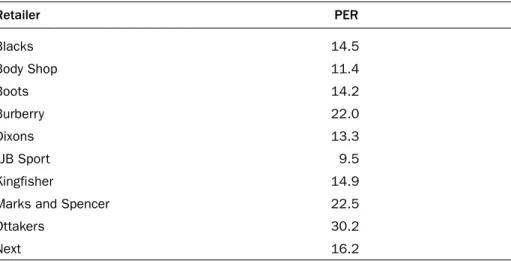
So, the retailer Dixons which reported earnings per share of 10.7p with a share price of £141.75 in January 2004 had a PER of about 13.3 (141.75/10.7p).
PERs of other retailers are shown in Table 13.3.
TABLE 13.3 PERs for retailers
Retailer PER
Blacks 14.5
Body Shop 11.4
Boots 14.2
Burberry 22.0
Dixons 13.3
JJB Sport 9.5
Kingfisher 14.9
Marks and Spencer 22.5
Ottakers 30.2
Next 16.2
Source: Financial Times, 10/11 January 2004
Investors are willing to buy Burberry’s shares at 22 times last year’s earnings compared with only 11.4 times last year’s earnings for Body Shop. One explana- tion for the difference in PERs is that companies with higher PERs are expected to show faster growth in earnings in the future. Burberry may appear expensive relative to Body Shop based on historical profit figures but the differential may be justified when forecasts of earnings are made. If a PER
is high investors expect profits to rise. This does not necessarily mean that all companies with high PERs are expected to perform to a high standard, merely that they are expected to do significantly better than
in the past. Few people would argue that Marks and Spencer has performed, or will perform, well in comparison with Burberry and yet it stands at a higher his- toric PER, reflecting the market’s belief that Marks and Spencer has more growth potential from its low base than Burberry.
PERs are also influenced by the uncertainty of the future earnings growth.
So, perhaps, Dixons and Kingfisher might have the same expected growth rate but the growth at Dixons is subject to more risk and therefore the market assigns a lower earnings multiple.
PERs over time
There have been great changes over the years in the market’s view of what is a reasonable multiple of earnings to place on share prices. What is excessive in one year is acceptable in another. This is illustrated in Figure 13.2.
If a PER is high investors expect profits to rise.
50
000s
70 45
15 10 5 0
72 74 76 78 80 82 84 86 88 90 92 94 96 98 00 02
UK-DS MARKET – PER S&P 500 COMPOSITE – PER 40
35 30 25 20
FIGURE 13.2
PERs for the UK and US (S&P 500) stock markets 1970–2004
Source: Thomson Financial Datastream
The crude and the sophisticated use of the PER model
Some analysts use the historic PER (P0/E0), to make comparisons between firms without making explicit the considerations hidden in the analysis. They have a view of an appropriate PER based on current prevailing PER for other firms in the same industry. So, for example, in 2004 Tesco with a PER of 17.5 may be judged to be priced correctly relative to similar firms – Sainsbury had a PER of 13.3, Morrisons 20.1 and Big Food Group 14. Analyzing through comparisons lacks intellectual rigor.
First, the assumption that the ‘comparable’ companies are correctly priced is a bold one. It is easy to see how the market could be pulled up (or down) by its own bootstraps and lose touch with fundamental considera- tions by this kind of thinking (say, telecommunication shares in the 1998–2000 bubble). Second, it fails to provide a framework for the analyst to test the important implicit input assumptions – for example, the growth rate expected in earnings in each of the companies, or the difference in required rate of return given the different risk level of each. These elements are probably in the mind of the analyst, but there may be benefits in making these more explicit.
This can be done with the more complete PER model, which is forward-looking and recognizes both risk levels and growth projections.
The infinite dividend growth model can be used to develop the more com- plete PER model because they are both dependent on the key variables of growth, g(in dividends or earnings), and the required rate of return, kE. The dividend growth model is:
d1 P0= ––––––
kE– g
If both sides of the dividend growth model are divided by the expected earn- ings for the next year, E1, then:
P0 d1/E1 ––– = ––––––
E1 kE– g
Note this is a prospectivePER because it uses next year’s earnings E1, rather than an historic PER, which uses E0.
In this more complete model the appropriate multiple of earnings for a share rises as the growth rate, g, goes up; and falls as the required rate of return, kE, increases. The relationship with the ratio d1/E1is more complicated. If this payout ratio is raised it will not necessarily increase the PER because of the impact on g– if more of the earnings are paid out less financial resource is being invested in projects within the business, and therefore future growth may decline.
Analyzing through comparisons lacks intellectual rigor.
Worked example 13.4 RIDGE PLC
Ridge plc is anticipated to maintain a payout ratio of 48% of earnings. The appropriate discount rate for a share for this risk class is 14% and the expected growth rate in earnings and dividends is 6%.
P0 d1/E1 ––– = ––––––
E1 kE– g P0 0.48
––– = ––––––––––– = 6 E1 0.14 – 0.06
The spread between kEand g is the main influence on an acceptable PER. A small change can have a large impact. Taking the case of Ridge, if we now assume a kEof 12% and gof 8% the PER doubles.
P0 0.48
––– = ––––––––––– = 12 E1 0.12 – 0.08
If kEbecomes 16% and g4% then the PER reduces to two-thirds its former value:
P0 0.48
––– = ––––––––––– = 4 E1 0.16 – 0.04
Worked example 13.5 WHIZZ PLC
You are interested in purchasing shares in Whizz plc. This company pro- duces high-technology products and has shown strong earnings growth for a number of years. For the past five years earnings per share have grown, on average, by 10% per annum.
Despite this performance and analysts’ assurances that this growth rate will continue for the foreseeable future you are put off by the exceptionally high prospective price earnings ratio (PER) of 25.
In the light of the more complete forward-looking PER method, should you buy the shares or place your money elsewhere?
Whizz has a beta of 1.8 which may be taken as the most appropriate sys- tematic risk adjustment to the risk premium for the average share (see Chapter 10).
The risk premium for equities over government bonds has been 5% over the past few decades, and the current risk-free rate of return is 7%.
Whizz pays out 50% of its earnings as dividends.
Prospective PER varies with g and kE
If an assumption is made concerning the payout ratio, then a table can be drawn up to show how PERs vary with kEand g.
A payout ratio of 40–50 percent of after tax earnings is normal for UK shares, although in periods of profit declines companies tended to maintain dividends thus pushing up the proportion of earnings paid out to around 60 percent.
Answer
Stage 1 Calculate the appropriate cost of equity kE= rf+ β(rm– rf) kE= 7 + 1.8 (5) = 16%
Stage 2 Use the more complete PER model P0 d1/E1 0.5
––– = ––––– = –––––––––– = 8.33 E1 kE– g 0.16 – 0.10
The maximum multiple of next year’s earnings you would be willing to pay given the growth rate of dividends hereafter of 10% is 8.33. This is a third of the amount you are being asked to pay, therefore you will refuse to buy the share.
d1 Assumed payout ratio = –– = 0.5
E1 Discount rate, kE
8 9 10 12
Growth 0 6.3 5.6 5.0 4.2
rate, g 4 12.5 10.0 8.3 6.3
5 16.7 12.5 10.0 7.1
6 25.0 16.7 12.5 8.3
8 – 50.0 25.0 12.5
FIGURE 13.3
Prospective PERs for various risk classes and dividend growth rates
The more complete model can help explain the apparently perverse behavior of stock markets. If there is ‘good’ economic news such as a rise in industrial output or a fall in unemployment the stock market often falls. The market likes the increase in earnings that such news implies, but this effect is often out- weighed by the effects of the next stage. An economy growing at a fast pace is vulnerable to rises in inflation and the market will anticipate rises in interest rates to reflect this. Thus the rfand the rest of the SML are pushed upward. The return required on shares, kE, will rise, and this will have a depressing effect on share prices. The article reproduced in Exhibit 13.5 expresses this well.
Payout ratio
Superficially P0 relative to E1 could be raised by increasing payout ratio. However a lower retention ratio may reduce g to leave the overall value lower.
Growth rate, g
A complex composite of myriad influences on a firm’s future growth of earnings and dividends, e.g.:
• proportion of profit retained;
• efficient use of resources;
• market opportunities;
• quality of management;
• strategy.
P0
E1 = d1 kE
E1 g /
–
rm rf
Rate of return
SML
Systematic risk on average share
Systematic risk FIGURE 13.4
The more complete PER model makes explicit key elements hidden in the crude PER model
Note the influences on the risk- return relation: for example if prospective inflation rises, interest rates (probably) will rise and the SML shifts upwards thus increas- ing kE. Also the risk profile of the firm may change with a new strat- egy; therefore altering kE.
Required return, kE, related to risk class of share
Valuation using cash flow
The third and the most important valuation method is cash flow. In business it is often said that ‘cash is king’. From the shareholders’ perspective the cash flow relating to a share is crucial – they hand over cash and are interested in the abil- ity of the business to return cash to them. John Allday, head of valuation at Ernst and Young, says that discounted cash flow ‘is the purest way. I would prefer to adopt it if the information is there’.4
The interest in cash flow is promoted by the limited usefulness of published accounts. Skepticism about the accuracy of earnings figures, given the flexibility available in their construction, prompts a switch of attention to a purer valua- tion method than PER.
The cash flow approach involves the discounting of future cash flows. These cash flows are defined as the cash generated by the business after deduction of investment in fixed assets and working capital to fully maintain its long-term competitive position and its unit volume and to make investment in all new value-creating projects. To derive the cash flow attributable to shareholders, any interest paid in a particular period is deducted as well as taxation. The process of the derivation of cash flow from profit figures is shown in Figure 13.5.
EXHIBIT 13.5 Why policymakers should take note
Source: Financial Times, 5 February 1996.
Why policymakers should take note
Philip Coggan
One issue which always mystifies the novice investor is why the financial mar- kets always react so joyously to bad economic news. A rise in unemployment or a fall in industrial production seems to be worth a point on bonds and a jump in the stock market index.
Experienced global investors explain patiently that the key determinant of short term financial market performance is interest rates. Slower growth prompts monetary authorities to lower rates; this
in turn reduces corporate costs, reduces the appeal of holding cash, and in the case of falling long term yields, by low- ering the rate at which future income streams are discounted, increases the present value of shares.
Conversely, of course, faster eco- nomic growth causes governments and central banks to fear higher inflation, prompting them to increase interest rates, with consequent adverse effects on share prices.
An example of a cash flow calculation is shown in Table 13.4. The difference between profit and cash flows is particularly stark in the case of 2006 – the earn- ings number is much larger than the cash flow because of the large capital investment in fixed assets. Earnings are positive because only a small proportion of the cost of the new fixed assets is depreciated in that year.
Note also that there is a subtle assumption in this type of analysis. This is that all annual cash flows are paid out to shareholders rather than reinvested. If all positive NPV projects have been accepted using the money allocated to addi- tional capital expenditures on fixed assets and working capital, then to withhold further money from shareholders would be value destructive because any other
Discount back to the present the resulting annual cash flows attributable
to shareholders Interest payments
Tax paid Increases in working capital e.g. • rise in debtors
• rise in stocks
• rise in cash requirements Capital expenditure on fixed assets Start with projected pre-tax, pre-interest profits
Add back
Take away
Take away
Take away
Take away Depreciation Amortization and depletion FIGURE 13.5
Cash flow calculation from projected profit figures
projects would have negative NPVs. An alternative assumption, which amounts to the same effect in terms of share value, is that any cash flows that are retained and reinvested generate a return that merely equals the required rate of return for that risk class. If they produce merely the cost of capital no value is created. Of course, if the company knows of other positive value projects, either at the outset or comes across them in future years, it should take them up. This will alter the numbers in the table and so a new valuation is needed.
The definition of cash flow used here (which includes a deduction of expendi- ture on investment in fixed and working capital to maintain long-term competitive position, unit volume and make all new value creating projects) is significantly dif- ferent to many accountant’s and analyst’s definitions of cash flow. They often neglect to allow for one or more of these factors. Be careful if you are presented with alternative cash flow numbers based on a different definition of cash flow.
TABLE 13.4
Cash flow-based share valuation
£m 2005 2006 2007 2008 2009 Estimated average
annual cash flow for period beyond planning horizon 2010–infinity Forecast pre-tax, +11.0 +15.0 +15.0 +16.0 +17.0
pre-interest profits
Add depreciation, +1.0 +2.5 +5.5 +4.5 +4.0 amortization and
depletion
Working capital +1.0 –0.5 0.0 +1.0 +1.0
increase (–) decrease (+)
Tax (paid in year) –3.3 –5.0 –5.0 –5.4 –5.8 Interest on debt –0.5 –0.5 –0.5 –0.6 –0.7 capital
Fixed capital –1.0 –16.0 0.0 –1.2 –1.8
investment
Cash flow +8.2 –4.5 +15.0 +14.3 +13.7 +14.0
Cash flow per 8.2p –4.5p 15p 14.3p 13.7p 14p
share (assuming 100m shares)
Discounted cash 8.2 4.5 15 14.3 13.7 14 1
–––– – –––––– + –––––– + –––––– + ––––––– + ––––– ×––––––
flow kE= 14% 1.14 (1.14)2 (1.14)3 (1.14)4 (1.14)5 0.14 (1.14)5 Share value = 7.20 –3.5 +10.1 +8.5 +7.1 +51.9
= 81.3p