DO NATURAL DISASTERS INCREASE FINANCIAL RISKS?
AN EMPIRICAL ANALYSIS
Chun-Ping Chang* and Wan-Li Zhang**
* Department of Marketing Management, Shih Chien University, Kaohsiung, Taiwan.
Email: [email protected]
** Corresponding Author. School of Economics and Finance, Xian Jiaotong University, Xian, Shaanxi, China.
Email: [email protected]
Using an unbalanced panel data consisting of deaths from natural disasters and five factors of financial risks in 136 countries, this paper analyzes the effect of natural disasters on different financial risks. The conclusions are as follows: (1) natural disasters lead to financial crisis by reducing GDP and trade and increasing domestic and foreign debt; (2) the effects of natural disasters on financial risks are dynamic and long term, with the effect weakening with time; and (3) the negative effects of natural disasters on financial risks in high-income and OECD countries are smaller than those of low-income and non-OECD countries.
Article history:
Received : July 15, 2019 Revised : October 20, 2019 Accepted : December 29, 2019 Available Online : January 2, 2020 https://doi.org/10.21098/bemp.v23vi0.1215
Keywords: Natural disaster; Financial risks; Fixed effects model; Panel unit root test.
JEL Classifications: E44; F30; O1; Q54.
ABSTRACT
I. INTRODUCTION
There is growing evidence that people’s lives are affected by climate change, such as increases in temperature and sea levels, aggravated environmental pollution, and decreases in forest cover area (Kabisch et al., 2016). For these reasons, the quantity and severity of natural disasters worldwide are rapidly rising. A natural disaster can influence the economy, finance, and politics via loss of life and property (Mohan et al., 2018). Different natural disasters also have different impacts on financial risks, including foreign debt, exchange rate stability, international liquidity, and the current account. When a natural disaster strikes, central and regional governments must increase investments and subsidies to rebuild and help casualties (Ward et al., 2020). Among the least developed countries, foreign debt will increase, as will the current account with growing demand, due to a decline in crop production. For countries with little land area and poverty problems, natural disasters can even cause civil war and disturbances, which can lead to a decline in exchange rates (Abarcar, 2017; Klomp, 2017). Organisation for Economic Co- operation and Development (OECD) countries can obtain assistance from member countries, which can help alleviate financial risks. In this regard, knowledge of the way a natural disaster affects financial risks is necessary. Whether a natural disaster has different influences on financial risks, given heterogeneity across countries, is also significant knowledge.
For instance, hurricane season creates problems for coastal countries, such as Jamaica and Grenada. According to Heger et al. (2008), hurricane losses reached almost US$3.1 billion in 2004, which is 10% of the Gross Domestic Product (GDP) of Jamaica and 200% of the GDP of Grenada. Such losses have forced the government of Grenada to provide fewer subsidies to its inhabitants. Such a decline in living standards will reduce both savings and investments, which is not conducive to the development of financial sectors, and financial risks will thus increase. The International Monetary Fund (IMF, 2003) has concluded that the damage caused by natural disasters contributes 3% of the fiscal deficit in Africa (Strobl, 2012). The December 2004 Indian Ocean tsunami and Cyclone Nargis, which hit Myanmar in May 2008, also catastrophically damaged local economic and financial development (Barthel and Neumayer, 2012). These instances show how natural disasters have a strong influence on financial risks, with diverse effects for different countries.
How, then, do natural disasters affect financial risks? Why are there such big gaps in financial risks between different regions? To explain these issues, we must analyze the factors of the financial risks and consider different national characteristics. According to the International Country Risk Guide (ICRG), financial risks can be divided into five categories (Bayoumi et al., 2015).
First, it is obvious that earthquakes and tsunamis are the most influential natural disasters, since they both result in high mortality rates and severe building damage. Such destruction is catastrophic for small countries and can even destroy whole cities, which the country must rebuild by investing more money. However, the source of reconstruction funds is the national revenue and debt from other countries. National foreign debt thus increases and the countries will be unable to pay the debt service (Skoufias, 2003; Ouattara and Strobl, 2013). Second, although storms, flooding, and drought will not cause as many deaths or losses of homes, they will harm crops and their harvest. The GDP and exports will
decrease dramatically, especially for developing countries which depend mainly on agriculture, and the current account deficit will rise and result in exchange rate instability and depreciation of the national currency (Kilby, 2009; Baur et al., 2018). Third, heavy losses force countries to use foreign exchange reserves, which maintain exchange rate stability, to adjust the balance of payments and international liquidity. If the loss, as a percentage of the GDP, is small, however, the country will not need to use foreign exchange reserves. When a natural disaster strikes, OECD members will also help each other via humanitarian assistance, financial rescue, and rescue materials (Toya and Skidmore, 2007; Yamamura, 2014). This will reduce foreign debt and the current account, helping avoid financial risks. Overall, the evidence suggests that natural disasters have different effects on financial risks in countries of different economic levels. The relations also vary between OECD and non-OECD countries.
The objectives of this paper are twofold. The first objective is to collect data on natural disasters from EM-DAT, the international disasters database, and to recalculate the losses of natural disasters, to verify their impact on financial risks. Some of the literature studies only the effect of specific natural disasters on economic conditions (Jonkman and Kelman, 2005; Barone and Mocetti, 2014).
However, there are many types of natural disasters, such as earthquakes, floods, landslides, storms, epidemics, and tsunamis. All of these will affect financial risks, and the adoption of data on a specific natural disaster will significantly underestimate the impacts (Cassar et al., 2017).
This paper thus calculates the sum of the deaths from total natural disasters for different countries every year to study the relation between deaths caused by natural disasters and different financial risks. We also use the number of natural disasters as a control variable to measure the frequency of disasters. Many studies only analyze how natural disasters affect the exchange rate and foreign debt (Gourio, 2013; Farhi and Gabaix, 2015). Ebeke and Combes (2013) also use lagged measures of natural disasters to study their effect on output growth volatility.
They find natural disasters to have a sustained influence. Generally speaking, our research studies the dynamic effects of the total damage of natural disasters on different financial risks. We conclude that the total death count has a negative effect on all financial risks.
The second major objective of this paper is to explore the effect of natural disasters on financial risks among OECD countries and countries with different income levels. Earthquakes and tsunamis have a stronger influence on trade in coastal countries, such as Japan and Korea. Such disasters decrease exports and imports affecting global supply chains. OECD members will assist an OECD country that has suffered a disaster. If the losses as a percentage of the GDP are not large, the economy could return to normal within weeks, with financial risks gradually returning to stability (Schettkat, 2010; Waldenberger, 2013). The negative relation between natural disasters and financial risks in OECD countries could be smaller than in non-OECD countries. Kellenberg and Mobarak (2008) propose that rising incomes will reduce the impact of natural disasters. Raddatz (2007) points out that natural disasters have a short-run impact on economics. Middle-income countries undergo a big impact and need a long time to recover. Kim (2012) finds that, in the 21st century, people in poor countries are twice as exposed to natural disasters
than in high-income countries. Countries with different income levels suffer from different levels of damage from natural disasters, and natural disasters also have diverse impacts on financial risks. Therefore, this article divides countries into two subsamples, namely, countries categorized by income level (high- and low- income countries) and countries categorized by whether they are OECD members or not, to analyze the different dynamic relations.
Summarizing the abovementioned literature, there are many studies on the impacts of different natural disasters and how they affect politics and economics.
However, very few studies have focused on the relation between natural disasters and financial risks. Moreover, the dynamic relation between natural disasters and financial risks is seldom considered together with heterogeneity across countries. In addition, this paper makes three contributions to the literature, as follows. (1) Unlike other research on the effects of natural disaster on financial risks, our work focuses on financial risks along the following five dimensions:
total foreign debt, debt service, the current account, international liquidity, and exchange rate stability. This method allows us to understand the total influence of natural disasters on different financial risks. (2) We split the full sample into two subsamples based on OECD membership and income levels according to the World Bank’s classification. We test whether low-income and non-OECD countries face more severe financial risks (Raddatz, 2007; Hallegatte et al., 2013).
(3) The previous literature has found that natural disasters have long-term effects.
Nevertheless, there is little research that investigates the relation between natural disasters and financial risks with regard to time effects and heterogeneity across countries simultaneously (Berrebi and Ostwald, 2013; Toya and Skidmore, 2014).
This paper studies the dynamic effect of natural disasters on different financial risks together with consideration of OECD membership and income levels.
The remainder of the paper is organized as follows. Section II presents the data and methodology. Section III shows the parameter estimation based on panel fixed effects regression and analyzes the results considering OECD membership and different income levels. Finally, Section IV summarizes the results and offers policy suggestions.
II. DATA DESCRIPTION AND METHOD A. Methodology
To test whether natural disasters affect financial risks, we first use the following empirical framework:
where , the main dependent variable, represents the different financial risks; is the independent variable, proxied by the total number of death due to natural disasters; stands for the number of natural disasters; and represents the control variables. In Equation (1), captures the individual countries’ fixed effects, captures time fixed effects, the term is the residual of the model, and indicates the five types of financial risks, with t=1,2,...,T periods and (1)
i=1,2,...,N panel members. This paper uses panel fixed effects regression to estimate the parameters.
In Equation (1), β, which is the coefficient of , shows the magnitude of the effect of natural disasters on financial risks. The role of is to illustrate how the frequency of natural disasters affects finance. It is generally accepted that a country with a large area and high population density can be subject to serious damage from a natural disaster. Hence, this paper uses the frequency of natural disasters. Miao and Popp (2014) point out that natural disasters have a long-term impact on economics. We therefore add the lagged terms of natural disasters into the equation and obtain the following new model:
where represents the lagged rank of the independent variable, represents the effect of a natural disaster on current financial risks, and and indicate whether current financial risks are influenced by natural disasters in the two previous years. This model considers the dynamic effects of natural disasters and provides a better explanation than static panel model.
B. Data Set
B.1. Dependent Variables
This paper analyzes how natural disasters affect different financial risks. We categorize the financial risks, as the dependent variables, into the five following factors, according to the ICRG classification (Byoun and Xu, 2014; Chiu and Lee, 2019).
(1) Total foreign debt (Risk1). This variable is measured by the ratio of gross foreign debt to the gross domestic product, where all terms are converted into US dollars at the average exchange rate for that year. The values range from zero to 10. The country faces less serious financial risks when total foreign debt increases.
(2) Debt service (Risk2). This variable is assessed by foreign debt service as the percentage of total exports of goods and services, where all terms are converted into US dollars at the average exchange rate for that year. The values range from zero to 10. As debt service increases, financial risks gradually decrease.
(3) Exchange rate stability (Risk3). This variable is calculated by the value of the appreciation or depreciation of the currency against the US dollar (against the euro in the case of the United States) over a 12-month period. The value ranges from zero to 10. Its implication is the same as debt service’s (Risk2), namely, that financial risks increase if the exchange rate stability decreases.
(4) Current account (Risk4). This variable is measured by the ratio of the balance of payments to the sum of the total exports of goods and services, where both terms are converted into US dollars. The magnitude of this variable ranges from zero to 15. Financial risks decrease with the increasing value of the current account.
(5) International liquidity (Risk5). This variable is assessed by the proportion of official holdings of gold to the average monthly merchandise import cost, where (2)
both terms are converted into US dollars. It should be noted that this index excludes IMF credits and the foreign liabilities of the monetary authorities. It provides a comparative liquidity risk ratio that indicates how many months of imports can be financed with reserves. The index ranges from zero to five. The greater the value of international liquidity, the smaller the financial risks.
B.2. Independent Variables
This paper uses the impact of natural disasters as the independent variable, namely, the number of deaths from disasters and the total number of persons affected, to study the relation between natural disasters and financial risks. To control for the influence of natural disasters’ frequency and distinguish large disasters from small ones, we use an index for the number of disasters every year (Visser et al., 2014; Ward and Shively, 2017). Generally speaking, Ndd, Nde, and Ndn are the logarithms of the numbers of deaths, the total number of persons affected, and the number of disasters, respectively. We also use one- and two- period lags of the three independent variables to analyze the dynamics. We use Ndd in the basic model and Nde in a robustness test and find they all have negative effects on financial risks. The types of natural disasters are obtained from EM-DAT and include droughts, earthquakes, epidemics, extreme temperatures, storms, landslides, floods, and volcanic eruptions. These indicators directly reflect the severity of natural disasters.
B.3. Control Variables
An additional issue is the role of other variables, which can influence financial risks. This paper controls for all such variables, as follows. (1) We use the GDP per capital (Pgdp) to measure the national income per capita, converted into US dollars.
Countries with a high income level generally have a more mature financial market and well-appointed infrastructure, which helps to reduce financial risks and avoid damage from natural disasters (Cavallo et al., 2013; Robinson et al., 2017). (2) We use net inflows of foreign direct investment (FDI), measured by the ratio of net inflows of foreign direct investment to the GDP, with all terms converted into US dollars. A higher FDI value indicates better development in the country, along with a higher GDP, a more skilled labor force, and so forth, all of which reduce financial risks (Hoshi, 2018; Pek et al., 2018). (3) Following Niepmann and Schmidt-Eisenlohr (2017), we use the ratio of imports and exports of goods and services to the GDP (Trade), converted into US dollars, to measure trade levels (Laseen et al., 2017).
(4) Song et al. (2018) point out that the uncertainty of research and development (R&D) requires strong financial support and low financial risk. Improper R&D expenditures will increase financial industrial business risk, financing risks and so on, throughout innovation failure and financing failure. We use the percentage of R&D expenditures to the GDP (R&D), following Li et al. (2019). (5) The ratio of the central government’s debt to the GDP (Gd) is used to measure a country’s debt level. Excessive government debt will increase pressure on the payments of financial institutions and enterprises (Liang et al., 2017). Note that foreign debt differs from central government debt. (6) We also follow Eckstein et al. (2019),
who conclude that financial risks increase when the unemployment rate rises. We thus use the ratio of unemployment to the total labor force (Unem) to assess the level of unemployment (Hall, 2017). (7) Zhang et al. (2016) indicate that the rapid expansion of manufacturers will exacerbate the misallocation of resources and lead to an unbalanced industrial structure, further exposing the whole economic sector to high risks. The industrial structure is thus introduced into the model and is calculated as value-added manufacturing to the value added of agriculture (Is). (8) It is obvious that inflation is the main instrument of monetary policy for controlling the economy (Fouejieu, 2017). However, unsuitable monetary policy will lead to a high inflation rate, as well as depreciation of the local currency.
National consumption will then surge, which will lead to high unemployment due to depreciation. The increasing foreign debt and unstable exchange rate will all increase financial risks. Hence, this paper adopts an inflation rate that considers a GDP deflator (IR). (9) The exchange rate, as a unit of measure of the national currency, can reflect national development. The exchange rate’s depreciation means the local currency is losing value, and residents will increase their investment in foreign exchange and fixed assets, increasing financial risks as well. We introduce the exchange rate (Er) into the model, following Reboredo et al. (2016). (10) Income inequality implies improper income distributions, industrial structures, and financing policies. Such lack of suitability will cause different levels of demand for imports and exports, which will affect the flow of international capital irrationally, as trade surplus or deficit will grow too large. Therefore, this paper utilizes the Gini index (Gini) to represent income inequality (Chiu and Lee, 2019).
C. Descriptive Statistics
First, we introduce the source of the data for this paper. The data on natural disasters are from EMDAT. The source of the financial risk data is ICRG. The data for the control variables are from World Bank Open Data. All the variables cover from 1984 to 2017, except Risk3, which ranges from 1984 to 2013. The sample is an unbalanced panel, since we delete missing values. World Bank Open Data divides countries into four categories: low income, lower middle income, upper middle income, and high income. In this paper, upper-middle-income and high-income countries are categorized as high-income countries. Low-income and lower- middle-income countries are categorized as low-income countries. Where are 136 countries in the sample, including 29 OECD and 107 non-OECD countries, with 88 high-income countries and 48 low-income countries.
The trends for Ndd and different financial risks are plotted in Figure 1. Note that Ndd and financial risks have opposite trends, suggesting a potentially negative relation between deaths due to natural disasters and different financial risks. Table 1 shows the descriptive statistics for the variables in the 136 sample countries, revealing means for Risk1, Risk2, Risk3, Risk4, and Risk5 of 7.951, 5.859, 6.743, 11.009, and 1.886, respectively. We find that the mean of Risk5 is the smallest, which indicates the highest financial risk. There are 3,731 observations for Risk3 from 1984 to 2013. The standard deviations of all the dependent variables are small, showing little fluctuation among the financial risks. We note that the means of Ndd and Ndn are 1.507 and 1.557, respectively, which indicates that natural disasters
are relatively severe. The standard deviations of Ndd and Ndn are also small, meaning that the numbers of disasters and resulting deaths vary only slightly.
Finally, the standard deviations of the control variables are small, indicating that these variables have inconspicuous fluctuations and that there are differences between the variables, except for Gd, Ir, Is, Unem, and Gini.
Figure 1.
Natural Disasters and Different Risks in the World (1984-2017)
This figure shows the relationship between the death from natural disasters (Ndd) and different risks in the world (1984-2017). Ndd is the logarithm of the national average death from natural disasters. Risk 1 to Risk 5 are the logarithms of different financial risks.
12 10 8 6 4 2 0
15 12 9 6 3
0 1984 1985 1986 1987 1988 1989 1990 1991 1992 1993 1994 1995 1996 1997 1998 1999 2000 2001 2002 2003 2004 2005 2006 2007 2008 2009 2010 2011 2012 2013 2014 2015 2016 2017
Year
Ndd Financial Risks
Ndd Risk1 Risk2 Risk3 Risk4 Risk5
Table 1.
Summary Statistics
This table reports the summary statistics of the variables in our research, which is obtained using STATA 15. Column 1 has variable name. “N” in column 2 represents the total number of observations. “Mean”, “Std. Dev”, “Minimum”,
“Maximum” and “Median” denote the descriptive statistics.
Variable N Mean Std. Dev Minimum Maximum Median
Risk1 4275 7.951 2.328 1.083 10.000 9.000
Risk2 4275 5.859 2.410 0.000 10.000 6.000
Risk3 3731 6.743 3.364 0.000 10.000 8.000
Risk4 4275 11.009 2.451 0.000 15.000 11.5
Risk5 4275 1.886 1.493 0.000 5.000 1.792
Ndd 4275 1.507 2.228 0.000 8.113 0.000
Ndn 4275 1.557 2.459 0.000 14.000 1.000
Pgdp 4275 1.042 1.485 0.251 6.965 0.366
FDI 4275 0.033 0.055 0.000 0.361 0.174
Trade 4275 3.912 1.225 0.123 5.797 4.162
R&D 4275 0.383 0.749 0.021 3.340 0.121
III. EMPIRICAL RESULTS A. Unit Root Test
Since the time span of our sample is relatively long, we first conduct a panel unit root test to ensure the robustness of the empirical results. We use a Fisher test to check the unit root, given the unbalanced panel of sample data (Fang and Chang, 2016). The unit root test assumes separate cross sections (Sadorsky, 2014). Pesaran (2007) indicates that the unit root test will be invalid with significant deviations as long as panel data correlation exists among the cross-sectional data. Therefore, we conduct a cross-sectional dependence test, following Pesaran (2007) and Wei et al. (2019). We also remove the means of cross-sectional units before running a Fisher test. Table 2 shows the final results. It is obvious that the cross-sectional dependence tests of all the variables can be significantly rejected at the 1% level, revealing cross-sectional correlation. Therefore, the panel unit test is valid. The panel unit root test and second panel unit root test results show that all the variables, except for Ex, are rejected at the 1% level. Therefore, there is no unit root.
Table 1.
Summary Statistics (Continued)
Variable N Mean Std. Dev Minimum Maximum Median
Gd 4275 11.954 27.098 1.792 129.874 2.165
Unem 4275 6.370 5.547 2.143 24.439 5.280
Is 4275 4.319 9.886 0.458 75.452 1.438
Ir 4275 13.153 34.103 -12.994 276.754 4.789
Ex 4275 0.039 0.146 0.001 1.103 0.006
Gini 4275 11.428 18.595 0.001 58.100 0.125
Table 2.
Cross-Section Correlation Test and Panel Unit Root Test
This table shows the cross-section correlation test and panel unit root test for all variables. These tests are performed by using STATA 15. The CD-test follows the research of Wei et al. (2019) and the original hypothesis is that there exists a cross-section correlation. The fisher-test follows the research of Fang and Chang (2016) and the original hypothesis is that there exists panel unit root.
Variable Cross-section correlation Panel unit root Second Panel unit root CD-test p-value Fisher-test p-value CIPS-test p-value
Risk1 275.009 0.00 50.379 0.00 -4.155 0.00
Risk2 23.366 0.00 24.538 0.00 -4.356 0.00
Risk3 420.638 0.00 40.508 0.00 -3.956 0.00
Risk4 43.508 0.00 50.128 0.00 -1.765 0.01
Risk5 60.808 0.00 30.199 0.00 -1.903 0.00
Ndd 16.509 0.00 57.432 0.00 -2.139 0.00
Ndn 37.29 0.00 51.999 0.00 -4.361 0.00
Pgdp 418.898 0.00 16.951 0.00 -2.404 0.00
FDI 106.621 0.00 24.905 0.00 -3.132 0.00
Trade 126.527 0.00 30.048 0.00 -2.928 0.00
R&D 113.801 0.00 30.703 0.00 -4.606 0.00
Variable Cross-section correlation Panel unit root Second Panel unit root CD-test p-value Fisher-test p-value CIPS-test p-value
Gd 24.759 0.00 31.703 0.00 -1.988 0.00
Unem 291.955 0.00 31.191 0.00 -2.803 0.00
Is 122.835 0.00 27.099 0.00 -3.056 0.00
Ir 81.843 0.00 44.475 0.00 -3.406 0.00
Ex 155.973 0.00 -1.328 0.90 -4.001 0.00
Gini 54.466 0.00 61.887 0.00 -5.045 0.00
Table 2.
Cross-Section Correlation Test and Panel Unit Root Test (Continued)
B. Preliminary Analysis
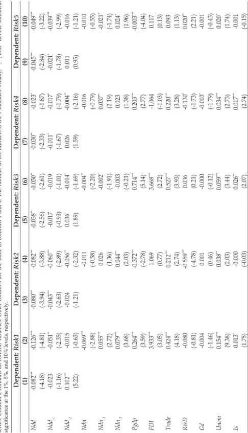
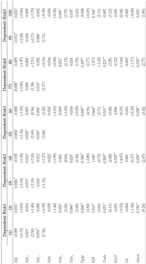
Table 3 displays the whole-sample estimation results for different financial risks.
The coefficient of deaths from natural disasters (Ndd) is negative and significant at the 10% significance level for different financial risks. Column (2) shows that the coefficients of Ndd-1 and Ndd-2 are -0.051 and -0.015, respectively, with t-test values of -2.35 and -1.21. This result means that the effects of natural disaster on foreign debt (Risk1) gradually become weaker and nonsignificant over time. The parameters of Ndn are also negative and significant. Column (4) shows that Ndd has a negative influence on debt service (Risk2), and the lagged terms have the same impact. It is obvious that the role of natural disasters on debt service also weakens with time. However, the coefficients of Ndn are nonsignificant. The Ndd variable affects exchange rate stability (Risk3) negatively in column (6), but the lagged terms are not significant. The Ndn variable also has a negative effect on exchange rate stability. The impacts of Ndd and Ndn decrease simultaneously.
From column (8), we obtain the same results, that the coefficient of Ndd on the current account (Risk4) is negative, with a nonsignificant t-test value of -1.87. The first lag of Ndd has a negative but significant effect, which indicates that the effect of Ndd is decreasing. Meanwhile, Ndn has a nonsignificant negative influence on the current account. Finally, column (10) shows that the parameters of Ndd and its lagged terms are -0.049, -0.039, and -0.016, respectively. There exists a negative impact on international liquidity (Risk5) to the Ndd that is gradually diminishing.
Although the effects of Ndn and its lagged terms are nonsignificant, they are also negative.
Table 3. Panel Fixed Effect Estimation of All Sample The table shows the dynamic estimation of all regressions via panel fixed effects. The regressions are run using STATA 15. Column 1 contains the independent variables and lagged terms. Column 2 contains all controll variables. Other columns are the same as columns 1 and 2. The number in the brackets is the t-statistics. Finally, ***, **, and * denote statistical significance at the 1%, 5%, and 10% levels, respectively. Dependent: Risk1Dependent: Risk2Dependent: Risk3Dependent: Risk4Dependent: Risk5 (1)(2)(3)(4)(5)(6)(7)(8)(9)(10) Ndd-0.082***-0.126***-0.080***-0.082***-0.038**-0.050**-0.030**-0.023*-0.045***-0.049*** (-4.18)(-4.81)(-3.94)(-3.88)(-2.56)(-2.61)(-2.33)(-1.87)(-2.84)(-3.22) Ndd-1-0.023-0.051**-0.043***-0.060***-0.017-0.019-0.011*-0.017*-0.021*-0.039*** (-1.16)(-2.35)(-2.63)(-2.89)(-0.93)(-1.01)(-1.67)(-1.79)(-1.78)(-2.99) Ndd-20.102***-0.015-0.024-0.056**0.036*-0.014*0.026-0.004**0.011-0.016 (5.22)(-0.63)(-1.21)(-2.32)(1.89)(-1.69)(1.59)(-2.16)(0.95)(-1.21) Ndn-0.069***-0.011-0.004**-0.016-0.010 (-2.88)(-0.58)(-2.20)(-0.79)(-0.55) Ndn-10.055***0.026-0.002*0.037**-0.021* (2.72)(1.36)(-1.91)(2.19)(-1.74) Ndn-20.079***0.044**-0.0030.0230.024* (3.68)(2.03)(-0.21)(1.38)(1.96) Pgdp0.264***-0.372***0.714***0.203***-0.003*** (3.59)(-2.78)(5.14)(2.77)(-4.04) FDI3.933***1.0693.668***-1.0640.117 (3.05)(0.77)(2.72)(-1.03)(0.13) Trade0.424***0.212***0.527***0.220***0.093 (4.18)(2.74)(3.93)(3.28)(1.13) R&D-0.080-0.559***0.036-0.130*0.020** (-0.81)(-4.78)(0.21)(-1.73)(2.21) Gd-0.0040.001-0.000-0.003*-0.001 (-1.46)(0.46)(-0.12)(-1.79)(-0.43) Unem0.154***0.038**0.059***0.034***0.020* (9.38)(2.03)(3.44)(2.73)(1.74) Is0.013*-0.0000.026**0.017***-0.001 (1.75)(-0.03)(2.07)(2.74)(-0.15)
Summarizing the above-mentioned results, we find that natural disasters have a negative influence on different financial risks and the dynamic relations are long term, with diminishing effects over time. A high number of deaths means that a disaster has caused catastrophic harm to the country. If a center of economic development is hard hit by a natural disaster, an economic crisis can be caused, including unemployment, factory closures, and riots. The government will increase domestic and foreign debt to assist those affected, which also leads to a decline in national comparative advantages. Devaluation of the domestic currency will cause the outflow of foreign currency and R&D, along with exchange rate instability. The country will also use foreign exchange reserves to promote local development and provide emergency assistance. In addition, natural disasters increase financial risks (Ajide and Raheem, 2016; Klomp, 2017). However, the living standards of the local residents and industrial development will gradually improve. along with the process that the country maintains to help affected areas.
People will regain confidence in reconstruction, and the global chain will continue to recover. Generally speaking, trade, the local currency, and investment will gradually stabilize, leading to decreases in financial risks over time.
C. Empirical Analysis of Heterogeneity
C.1. Classification by OECD and non-OECD Countries
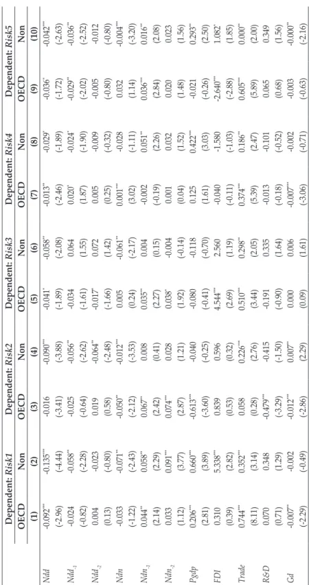
Table 4 shows the dynamic estimations for OECD and non-OECD countries.
Almost all of the variables are negative at the 10% level of significance. First, the coefficients of deaths from natural disasters (Ndd) for OECD and non-OECD countries are -0.092 and -0.135, respectively, with t-test values of -2.96 and -4.44.
This means that natural disasters have a negative effect on foreign debt (Risk1), and the influence in OECD countries is lower than that in non-OECD countries.
Furthermore, the lagged terms are decreasing over time, and Ndn follows the same trend as Ndd. Second, Ndd has a nonsignificantly negative relation with debt service (Risk2) among OECD members, but a significantly negative effect among non-OECD members. We arrive at the same conclusion, that the influence in OECD countries is smaller than in non-OECD countries, and the impact decreases gradually. Third, columns (5) and (6) indicate that the negative effect of Ndd on the exchange rate (Risk3) in OECD countries is also lower than in non-OECD countries, both with significant values. With time, the negative effect is gradually weakened. Fourth, the parameter of Ndd in OECD countries, in column (7), is -0.013, while the value in column (8) is -0.029. Both have a significant negative influence on the current account (Risk4). The trend of Ndd is the same as that of the other financial risks mentioned above. Finally, the coefficient of Ndd in OECD countries, namely, -0.036, is obviously smaller than that in non-OECD countries, at -0.042. The effects of natural disasters on international liquidity (Risk5) decrease over time in both OECD and non-OECD countries. Note that the parameters of the two lags of deaths from natural disasters are almost nonsignificant, revealing that natural disasters only affect financial risks in the current year and the next.
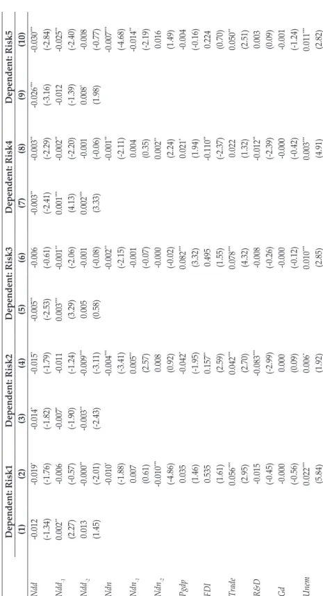
Table 4. Panel Fixed Effect Estimation of OECD and non-OECD Countries The table shows the dynamic estimation of OECD and non-OECD countries via panel fixed effect regressions. The regressions are performed by using STATA 15. The number in the brackets is the t-statistics. Finally, ***, **, and * denote statistical significance at the 1%, 5%, and 10% levels, respectively. Dependent: Risk1Dependent: Risk2Dependent: Risk3Dependent: Risk4Dependent: Risk5 OECDNonOECDNonOECDNonOECDNonOECDNon (1)(2)(3)(4)(5)(6)(7)(8)(9)(10) Ndd-0.092***-0.135***-0.016-0.090***-0.041*-0.058**-0.013**-0.029*-0.036*-0.042*** (-2.96)(-4.44)(-3.41)(-3.88)(-1.89)(-2.08)(-2.46)(-1.89)(-1.72)(-2.63) Ndd-1-0.024-0.058**-0.025-0.056**-0.0340.0640.020*-0.024*-0.029**-0.036** (-0.82)(-2.28)(-0.64)(-2.62)(-1.61)(1.55)(1.87)(-1.90)(-2.02)(-2.52) Ndd-20.004-0.0230.019-0.064**-0.017*0.0720.005-0.009-0.005-0.012 (0.13)(-0.80)(0.58)(-2.48)(-1.66)(1.42)(0.25)(-0.32)(-0.80)(-0.80) Ndn-0.033-0.071**-0.050**-0.012***0.005-0.061**0.001***-0.0280.032-0.004*** (-1.22)(-2.43)(-2.12)(-3.53)(0.24)(-2.17)(3.02)(-1.11)(1.14)(-3.20) Ndn-10.044**0.058**0.067**0.0080.035**0.004-0.0020.051**0.036***0.016** (2.14)(2.29)(2.42)(0.41)(2.27)(0.15)(-0.19)(2.26)(2.84)(2.08) Ndn-20.0330.091***0.074***0.0280.038*-0.0040.0010.0320.0200.023 (1.12)(3.77)(2.87)(1.21)(1.92)(-0.14)(0.04)(1.52)(1.48)(1.56) Pgdp0.206***0.660***-0.613***-0.040-0.080-0.1180.1250.422***-0.0210.293** (2.81)(3.89)(-3.60)(-0.25)(-0.41)(-0.70)(1.61)(3.03)(-0.26)(2.50) FDI0.3105.338***0.8390.5964.544***2.560-0.040-1.580-2.640***1.082* (0.39)(2.82)(0.53)(0.32)(2.69)(1.19)(-0.11)(-1.03)(-2.88)(1.85) Trade0.744***0.352***0.0580.226***0.510***0.298**0.374***0.186**0.605***0.000** (8.11)(3.14)(0.28)(2.76)(3.44)(2.05)(5.39)(2.47)(5.89)(2.00) R&D0.0700.348-0.479***-0.415-0.1910.335-0.013-0.1010.0650.349 (0.71)(1.29)(-3.29)(-1.50)(-0.90)(1.64)(-0.18)(-0.52)(0.68)(1.56) Gd-0.007**-0.002-0.012***0.007**0.0000.006-0.007***-0.002-0.003-0.000** (-2.29)(-0.49)(-2.86)(2.29)(0.09)(1.61)(-3.06)(-0.71)(-0.63)(-2.16)
Dependent: Risk1Dependent: Risk2Dependent: Risk3Dependent: Risk4Dependent: Risk5 OECDNonOECDNonOECDNonOECDNonOECDNon (1)(2)(3)(4)(5)(6)(7)(8)(9)(10) Unem0.0340.181***0.0060.052**0.051**0.045**0.033***0.037**-0.0250.029** (1.19)(9.31)(0.26)(2.35)(2.43)(2.02)(2.86)(2.34)(-1.56)(2.20) Is-0.0150.0080.055-0.0120.046***0.044**-0.0060.014**-0.014-0.006 (-0.90)(0.80)(1.69)(-0.69)(2.77)(2.18)(-0.39)(2.32)(-0.70)(-0.62) Ir-0.029***-0.016***-0.009**-0.008***-0.0030.003-0.001-0.005-0.011**-0.007*** (-4.32)(-6.10)(-2.33)(-4.44)(-1.26)(1.45)(-0.14)(-1.48)(-2.65)(-4.43) Ex-2.8651.337**6.8900.7852.861*-1.0355.459**2.333**11.6170.004*** (-1.35)(2.10)(1.59)(0.76)(1.90)(-0.65)(2.10)(2.03)(1.66)(3.01) Gini0.0040.009***-0.002-0.0020.009**0.009**-0.007**0.001-0.010**0.004* (0.93)(2.96)(-0.49)(-0.71)(2.43)(2.57)(-2.28)(0.60)(-2.35)(1.93) Cons5.103***4.693***8.331***4.792***4.868***4.845***9.973***9.552***-0.1021.612*** (14.58)(11.27)(9.18)(15.41)(8.44)(8.30)(34.61)(31.08)(-0.23)(5.20) N986328998632893847415998632899863289 R20.3640.3280.3480.0790.0960.0450.1030.0600.2490.120 Table 4. Panel Fixed Effect Estimation of OECD and non-OECD Countries (Continued)
Why, then, are the effects in OECD countries weaker than those in non- OECD countries? The OECD is an international intergovernmental economic organization that aims to jointly address economic and social problems caused by globalization. Compared with non-OECD countries, there is closer cooperation among OECD countries, including trade, global chain, and R&D activities.
Sometimes one OECD country will require the products of other OECD members as intermediate input. Those OECD countries that suffer natural disasters will influence the development of other OECD countries. To obtain intermediate input and technology, other OECD countries will provide assistance to disaster-affected members. Although natural disasters can cause many deaths and great economic loss, an OECD country can recover quickly with the help of other members (Holm and Østergaard, 2015; Breckner et al., 2016). Levels of trade, exchange rates, and foreign exchange reserves will remain stable to maintain financial risks. Moreover, OECD countries have more advanced economic development than non-OECD countries, including their GDP, financial market, and technology. If the loss as a percentage of the GDP is relatively small, countries will be able to offset the impact of natural disasters through domestic financial expenditures and humanitarian assistance.
C.2. World Bank Classification by Income
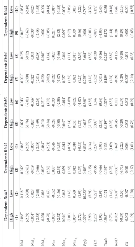
Kellenberg and Mobarak (2008) have pointed out that rising income will decrease the risk of damage from natural disasters. In addition, people with a high income tend to gain access to better infrastructure, safer places to live, and so on. Natural disasters thus have less of an effect on people’s lives, agriculture, and manufacture in countries with higher income levels. Therefore, this paper divides the whole sample into high- and low-income countries, following the World Bank’s classification. Table 5 shows the results for countries of different income levels.
We obtain the same conclusion, that natural disasters have a negative influence on different financial risks.
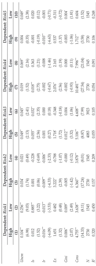
First, columns (1) and (2) in Table 5 show that the Ndd variable in high-income countries has a stronger negative effect on foreign debt (Risk1) than in low-income countries. The coefficients of Ndd are both significant, and the effect of Ndd decreases over time. Second, columns (3) and (4) show that the relations between Ndd and debt service (Risk2) are significantly negative, and the coefficients are -0.042 and -0.063, respectively. Natural disasters reduce the value of Risk2 and the negative effects weaken with time. Third, the coefficients of death from natural disasters (Ndd) for low- and high-income countries in columns (5) and (6), respectively, are -0.021 and -0.043, with t-test values of -1.76 and -2.01. The first lags of Ndd in different types of countries are all significantly negative, but less than the current coefficients. Fourth, we also arrive at the same results for the current account (Risk4), that the parameters of Ndd are all negative. The effect decreases significantly for high-income countries, but nonsignificantly for low- income countries. Finally, the relation between Ndd and international liquidity (Risk5) is the same as for other financial risks. The effects are significantly negative and weaken over time.
Table 5. Panel Fixed Effect Estimation of High-income and Low-income Countries The table shows the dynamic estimation of high-income and low-income countries via panel fixed effect regressions. The regressions are performed by using STATA 15. The number in the brackets is the t-statistics. Finally, ***, **, and * denote statistical significance at the 1%, 5%, and 10% levels, respectively. Dependent: Risk1Dependent: Risk2Dependent: Risk3Dependent: Risk4Dependent: Risk5 HighLowHighLowHighLowHighLowHighLow (1)(2)(3)(4)(5)(6)(7)(8)(9)(10) Ndd-0.068**-0.118***-0.042**-0.063**-0.021*-0.043**-0.001**-0.025-0.042***-0.054** (-2.59)(-3.00)(-2.61)(-2.09)(-1.76)(-2.01)(-2.00)(-0.52)(-3.62)(-2.48) Ndd-1-0.034**-0.028*-0.019-0.050**-0.026*-0.066**-0.022**0.003-0.030**-0.025* (-2.38)(-2.90)(-0.66)(-2.08)(-1.69)(2.26)(-2.01)(0.08)(-2.48)(-1.65) Ndd-2-0.0200.0160.016**-0.064**-0.0100.071***-0.0200.018***-0.002-0.008 (-0.78)(0.47)(2.56)(-2.21)(-0.34)(3.05)(-0.82)(3.44)(-0.08)(-0.44) Ndn-0.055**-0.0520.035**-0.046*-0.024-0.033**-0.022-0.025*0.021***-0.017** (-2.62)(-1.56)(2.61)(-1.65)(-0.88)(-2.58)(-1.07)(-1.66)(2.93)(-1.98) Ndn-10.044**0.0430.039-0.0130.049**-0.014*0.027*0.0400.029**0.001*** (2.01)(1.43)(1.63)(-0.54)(2.14)(-1.89)(1.87)(1.11)(2.07)(3.06) Ndn-20.057***0.068*0.042-0.0100.051*-0.0220.0220.011***0.0090.019 (2.72)(1.93)(1.57)(-0.45)(1.73)(-1.07)(1.25)(3.36)(0.66)(1.22) Pgdp0.279***10.232***-0.403***8.834***-0.613*0.568***0.225***3.661**-0.0015.787*** (3.99)(5.91)(-3.15)(4.14)(-1.77)(3.85)(3.16)(2.53)(-0.01)(4.37) FDI2.235*9.221***-0.9367.239***5.308**1.376-1.552**-0.630-0.8784.172** (1.92)(2.94)(-0.66)(3.91)(2.49)(0.86)(-2.01)(-0.16)(-1.03)(2.45) Trade0.563***0.1740.192**0.1330.419***0.376**0.189*0.243***0.172-0.050 (6.73)(1.46)(2.07)(1.09)(2.93)(2.52)(1.94)(2.82)(1.44)(-0.48) R&D-0.0622.438***-0.530***1.469**-0.0450.181-0.091-0.1150.0281.044** (-0.59)(3.55)(-4.71)(2.22)(-0.20)(1.09)(-1.29)(-0.18)(0.29)(2.13) Gd-0.003-0.007-0.0010.0060.0030.003-0.005**0.001-0.002-0.001 (-1.09)(-1.28)(-0.17)(1.61)(0.76)(0.99)(-2.14)(0.35)(-0.65)(-0.55)
Table 5. Panel Fixed Effect Estimation of High-income and Low-income Countries (Continued) Dependent: Risk1Dependent: Risk2Dependent: Risk3Dependent: Risk4Dependent: Risk5 HighLowHighLowHighLowHighLowHighLow (1)(2)(3)(4)(5)(6)(7)(8)(9)(10) Unem0.104***0.256***0.034*0.0210.049**0.045**0.0190.069**0.0040.049** (6.98)(9.03)(1.74)(0.49)(2.13)(2.41)(1.52)(2.16)(0.35)(2.38) Is0.0120.885***0.001-0.2280.055**0.032**0.018***0.363-0.0010.020 (1.52)(3.22)(0.06)(-0.69)(2.56)(2.35)(2.75)(1.21)(-0.19)(0.12) Ir-0.016***-0.013***-0.009***-0.006**0.0010.000-0.002-0.008-0.010***-0.001 (-6.09)(-3.53)(-4.33)(-2.33)(0.27)(0.18)(-0.67)(-1.46)(-6.63)(-0.71) Ex1.6510.4823.222**-0.7881.718*-0.3482.076**2.1650.537-0.311 (1.32)(0.48)(2.39)(-1.07)(1.72)(-0.18)(2.56)(1.19)(1.37)(-0.72) Gini0.006**0.009**-0.005-0.0000.012***0.004-0.0020.000-0.0030.004* (2.07)(2.49)(-1.42)(-0.12)(3.32)(1.06)(-0.93)(0.11)(-1.06)(1.81) Cons4.755***3.638***6.360***3.878***5.106***4.608***10.481***7.996***1.712***0.604 (14.33)(8.11)(17.24)(8.01)(8.87)(7.99)(27.54)(21.04)(3.58)(1.52) N2730154527301545408339232730154527301545 R20.3200.4500.1570.2090.0550.1050.0540.0910.1060.248