The evidence does not support acceptance of the self-dilution rule as a quantitative biological law. Self-thinning lines from forestry yield table data cited by previous authors in support of the self-thinning.
RMR 1-3
The importance of this general relationship with the rule of self-thinning for individual plant populations is considered. Several non-allometric explanations of the self-dilution rule have also been proposed.
CHAPTER 2
The possible ambiguity in the behavior of the model population below the zero isocline can be eliminated as follows. The first two terms of the right-hand side (RHS) of this equation simply give Equation 2.23 for the zero isocline.
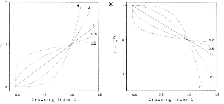
The equation associated with the first term on the RHS is simply equation 2.23 for the zero isocline of the basic model, while the remaining two terms give When two of the lines cross, the current zero isocline undergoes a gradual transition from one slope to the other.
Density (plants/m 2 )
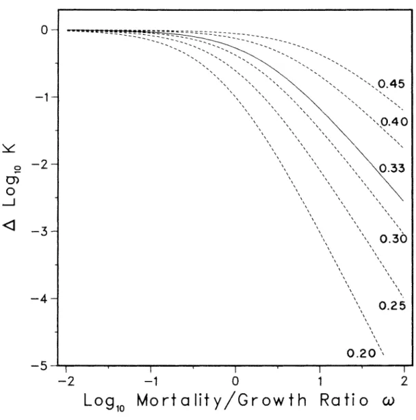
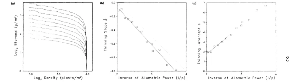
The slope of the model thinning line is determined only by the strength, p, of the area-weight relationship and is only equal to the classical thinning rule slope of B = -l/2 if p = 1/3. The position of the model's self-thinning line is also affected by the rate constants g0 and m, but these effects are relative.
Density (pI ants/ m 2 )
A survey sample taking over 0.5 ~log N ~ 1.5 from populations behaving as shown in Figure 2.5 would see virtually no difference between high light and reduced light paths. Confusion has arisen because the different studies have used different plants observed at different densities and thus focused on different areas of the overall behavior revealed in Figure 2.5.
CHAPTER 3
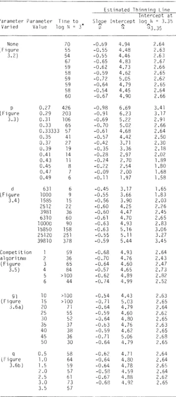
These effects arise because some plant competitors near the edge of the plot lie outside the plot and are not observed. The model was analyzed in three steps: (1) checking whether the dynamics resemble the actual self-dilution behavior, (2) evaluating the variations in the self-dilution trajectory solely due to. The time required for the density of individuals to drop from an initial value of 10,000 to 1,000 was recorded as a measure of the average rate of self-dilution.
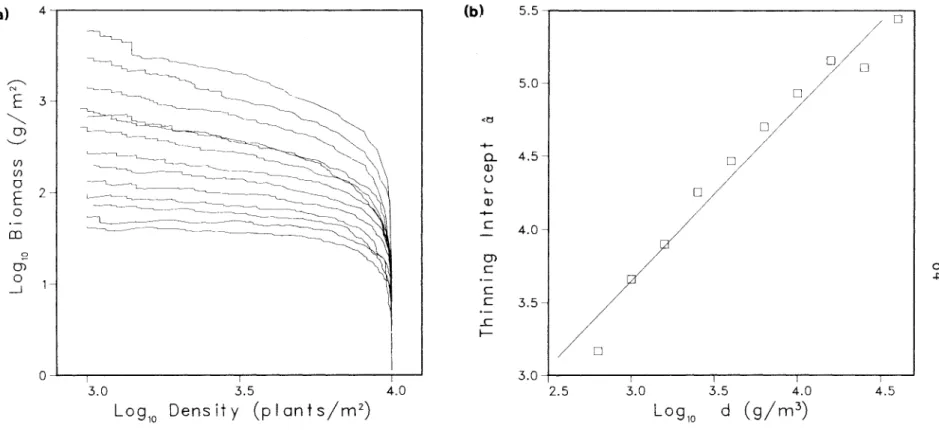
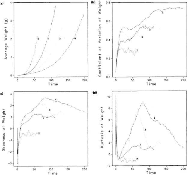
Typical dynamic behavior of the simulation model. a) is a self-diminishing log B-log N plot, (b) shows the logistic growth of total population biomass, and (c) shows approximately exponential mortality starting with the onset of thinning around time 20. log B-log N plot of simulations of the control group (Figure 3.2) shows that there are changes in the self-dilution trajectory that can only be attributed to the persistent effects of stochastic initial conditions. However, the slopes of the self-thinning lines are quite similar and the lines are all located within a narrow vertical band.
The parameter d, the density of biomass in the occupied space, influenced the position of the self-thinning line (Figure 3.4a), as measured by the thinning intercept a (rs = 0.99, p < 0.0001).
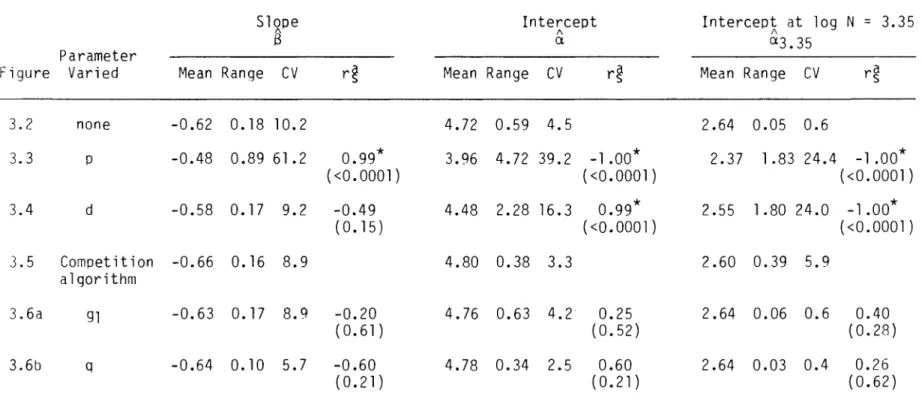
The lack of effect of the competing algorithm on slope thinning is indicated by the similar means and ranges for a in the control and experimental groups. The q = 3.5 simulation was not fitted with a dilution line, as the maximum weight limit came into effect before the linear part of the dilution path was established. Changes in the initial density also did not affect the position of the self-dilution line (Figure 3.6c}).
This analysis identified only one parameter, the power p related to the area occupied by the individual weight, that affected the slope of the model's self-thinning line. Environmental factors could then cause changes in the self-thinning line, not because the factors are important determinants of the thinning line, but because they influence the thinning line indirectly by changing the growth parameters of the plants. The significant effects of the competition algorithm on the rate of self-thinning and the position of the thinning line are… significant new results from this analysis.
Some results of this analysis are relevant to other theories about the causes of the self-dilution rule.
CHAPTER 4
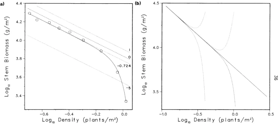
Another major difficulty in testing the self-thinning rule arises because the thinning line is an asymptotic limit that is approached only when stands become sufficiently crowded. To estimate the slope and position of the thinning line using linear statistics, data points from populations that are not constrained by the hypothetical linear constraint must be removed. Failure to eliminate such points will bias thinning estimates (Mohler et al. 1978), but when data are confounded with biological . variability and measurement errors, recognition and elimination.
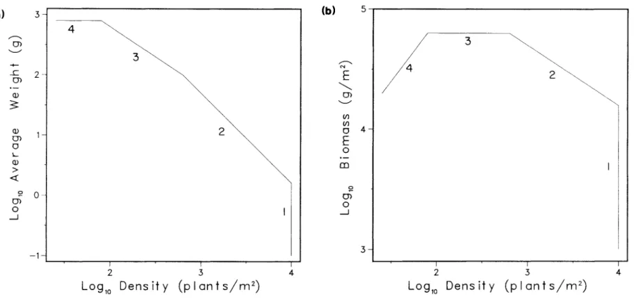
Because there is no prior estimate of the position of the thinning lines, decisions to eliminate data points must be made retrospectively (Westoby and Howell 1982). The sensitivity of thinning parameters to the choice of data points also has important statistical implications. Three examples of the sensitivity of self-thinning line parameters to the points chosen for analysis.
Three examples of the sensitivity of the self-diluting fitted line to points selected for analysis.
Density (pI ants/ m 2)
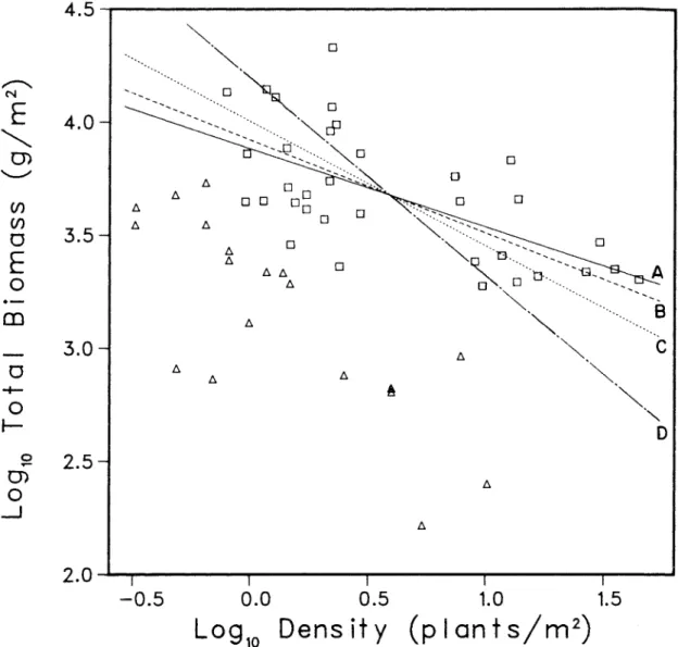
Another drawback of log ~-log N analysis is more serious and detrimental to the self-dilution rule: The misleading effects of this data transformation are present even in simple data plots. A log B-log N plot of the data (Chenopodium album, Yoda et al. 1963) shows an apparent linear constraint that could be estimated by fitting a line through the 13 square data points in Figure 4.6b.
When the artificial enhancement of linearity is removed upon examination of the log B-log N plot of (b), an apparent linear limitation is still visible; however, many data points fall relatively far from the limiting line (triangles). The log B-log N plot (b) shows the inadequacy of the straight line model for these data. A statistical test of the hypothesis that an observed thinning slope is equal to the predicted value provides a more objective test of agreement with the self-thinning rule.
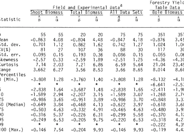
All FYD and 69 (91%) EFD rarefaction lines were estimated by relating log w to log N.
CHAPTER 5
Some single-species forest types were studied in both EFD and FYO. For EFD, the 95% confidence intervals for the thinning line parameters were compared to test for significant differences between the estimates. The predictions of the self-dilution rule have been tested here through five different analyses: (l) statistical tests of.
Seventy percent of the thinning lines showed the predicted significant linear relationship between log B and log N, but 32% of the thinning slopes were significantly different from S = -1 and did not agree quantitatively with the thinning rule. In fact, many data sets were too variable to be useful in resolving alternative hypotheses about the slope of the dilution line. Briefly, 30% of the datasets demonstrated none. The relationship between biomass and density, while another 32% quantitatively disagreed with the -1/2 slope predicted by the thinning rule.
The observed slope thinning departures from S = -1/2 for trees in EFO and FYD support Sprugel's (1984).
CHAPTER 6
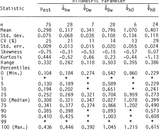
For example, the allometric equation n ~ w~hw can be fitted to measurements of mean height and mean weight of the same stands used to estimate a self-thinning slope. Of the 75 data sets in EFD that showed significant relationships between Log B and Log N (Chapter 5), 31 had companions. Two correlations between the transformed dilution slope and EFD allometric strengths were statistically significant.
Histograms of allometric powers of experimental and field data. a) through (f) show, respectively, the statistical distributions of the slope of the tra~formed !hinning, Pest' and the allometric powers $hw'. Allometric power histograms of forest yield table data. a) through (f) denote, respectively, the statistical distributions of the detailed slope, Pest• and the allometric powers ~hw•. Westoby (1976) tested the allometric derivation of the self-thinning rule by measuring the thinning slope of spreading cultivars of Trifolium subterraneum.
Several statistically significant relationships between the thinning slope and the allometric forces were found, but the most predictive one explained only 50% of the variation between the thinning slopes.
CHAPTER 7
7.2) The shape of the plants in a stand can be represented by the ratio between height and FULL radius, T = h/R. R = (TI N)- 112. The estimated R values can then be divided into the reported mean heights to obtain T, which ranges from 2 to 12 for Gorham's 65 stands. These two lines define a region of the log w-log N plane that includes all fully filled elevations of identical.
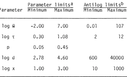
Since ln w is normally distributed, the ninety-ninth percentile value is 4.652 standard deviations above the first percentile value, and e4•652a = p. The values of the input parameters log T, p, log d, log w, and log p were selected from uniform random distributions on. The volume of any cylinder is a cubic function of the base radius, while the surface area of the base is a function of the same radius squared, so the ratio of these two powers is 3/2.
Variation ranges of variables derived in the Monte Carlo analysis of the improved model.
Density (plants/m 2)
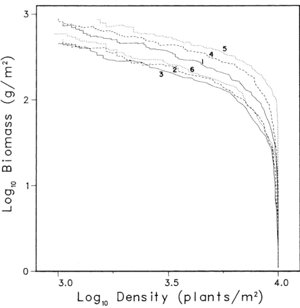
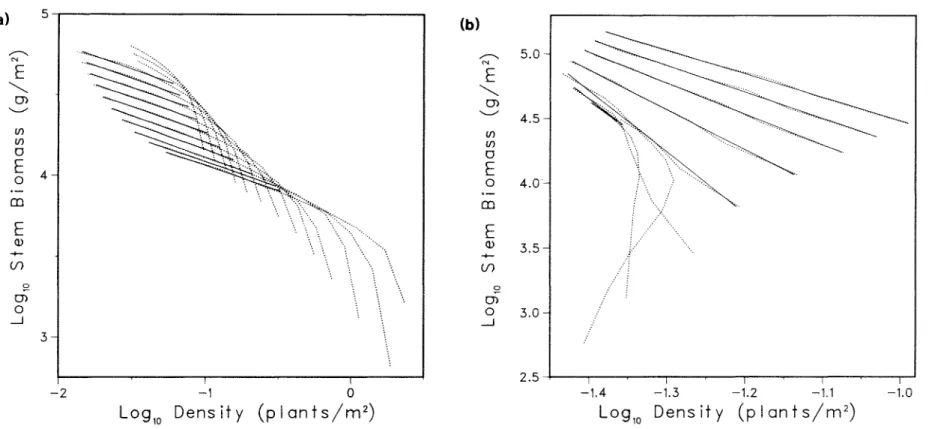
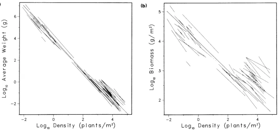
Because different phenomena are investigated, the existence of the overall relationship does not provide evidence for or against the self-dilution rule. However, the log B-log N plot of the same data (Figure 7.3b) with the dashed lines enclosing 90% of the observed stands shows that individual self-thinning lines can vary widely in slope and position from the overall trend, but still fall within the 90% limits. Previous analysis of the overall size-density relationship between thinning lines. a) shows 65 previously mentioned self-thinning lines drawn using a reported thinning slope and intercepts (Table A.5) over the range of log N values covered by the thinning line (Table A.3).
In (b), the same data and fitted line are shown in a log B–log N plot along with dashed lines enclosing 90% of the plant stands. Further verification of the models for the overall relationship can be achieved by comparing the predicted limits of variation. White (1981) stated that the limitation imposed by this ultimate thinning line demonstrates the importance of the self-thinning rule, even for species whose stand dynamics do not necessarily trace a line of slope −3/2 in the log w–log N plane.
Analysis by Mohler et al. 1978 ), which gave a slope close to −3/2, may have revealed a general relationship between stands along different thinning trajectories rather than a specific time trajectory of one of the stands.
CHAPTER 8 CONCLUSION